Python for Data Science
A Crash Course
Processing Tabular Data With pandas
Khalil El Mahrsi
2025

What is pandas?
- pandas is a powerful and intuitive Python package for tabular data analysis and manipulation
What Are Tabular Data?
- Tabular data are data that are structured into a table
What Are Tabular Data?
- Tabular data are data that are structured into a table (or data frame), i.e., into rows and columns
- Row → entities, objects, observations, instances
- e.g., patients, customers, students, plants, cars, houses, ...
- Column → variables, features, attributes
- e.g., age, gender, salary, ...
| Age | Job | Marital status | Housing | Loan default | |
|---|---|---|---|---|---|
| 1 | 30 | unemployed | divorced | no | yes |
| 2 | 35 | management | married | yes | no |
| 3 | 25 | services | single | no | no |
| 4 | 56 | management | divorced | yes | no |
| 5 | 22 | student | single | no | yes |
| 6 | 28 | unemployed | single | no | yes |
| 7 | 42 | unemployed | married | no | yes |
| ... | ... | ... | ... | ... | ... |
Variable Types

Quantitative (Numerical) Variables
- A quantitative variable has values that are numeric and that reflect a notion of magnitude
- Quantitative variables can be
- Discrete → finite set of countable values (often integers)
- e.g., number of children per family, number of rooms in a house, ...
- Continuous → infinity of possible values
- e.g., age, height, weight, distance, date and time, ...
- Math operations on quantitative variables make sense
- e.g., a person who has 4 children has twice as much children as a person who has 2
Qualitative (Categorical) Variables
- A qualitative variable's values represent categories (modalities, levels)
- They do not represent quantities or orders of magnitude
- Qualitative variables can be
- Nominal → modalities are unordered
- e.g., color,
- Ordinal → an order exists between modalities
- e.g., cloth sizes (XS, S, M, L, XL, XXL, ...), satisfaction level (very dissatisfied, dissatisfied, neutral, satisfied, very satisfied), ...
Encoding a categorical variable
with a numeric data type (e.g.,
int) does not make it
quantitative!
What is pandas?
- pandas is a powerful and intuitive Python package for tabular data analysis and manipulation
- Based on NumPy → many concepts (indexing, slicing, ...) work similarly
- Two main object types
-
DataFrame→ 2-dimensional data structure storing data of different types (strings, integers, floats, ...) in columns Series→ represents a column (series of values)
Installing and Importing pandas
Installing pandas with conda (recommended)
% conda install pandasInstalling pandas with pip
% pip install pandasImporting pandas (in Python scripts or notebooks)
>>> import pandas as pdBasic Functionalities
The Bank Marketing Data Set
- Most examples in this section use the Bank Marketing Data Set
- Variables
age: age in years (numeric)job: the customer's job category (categorical)marital:the customer's marital status (categorical)education: the customer's education level (ordinal)-
default: whether the customer has a loan in default (categorical) -
housing: whether the customer has a housing loan (categorical) -
loan: whether the customer has a presonal loan (categorical) - ...
-
y: how the customer responded to a marketing campaign (target variable)
Reading and Writing Data Frames
- CSV (comma-separated values) files are one of the most used formats for storing tabular data
-
Use the
read_csv()reader function to load a data frame from a CSV file -
Use the
to_csv()writer method to save a data frame to disk as a CSV file
Loading a DataFrame from a CSV file
df = pd.read_csv(file_path, sep=separator, ...) # sep defaults to ","Saving a DataFrame to a CSV file
df.to_csv(file_path, ...)
pandas also provides
reader and writer functions
for handling other popular formats (e.g., JSON, parquet, Excel, ...).
Head and Tail Methods
-
Use the
head()andtail()methods to view a small sample of aSeriesorDataFrame
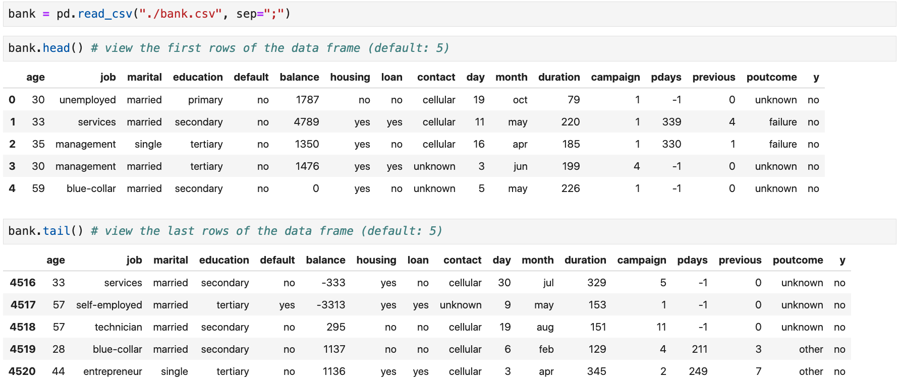
These methods are very useful to check
that you imported a data frame correctly.
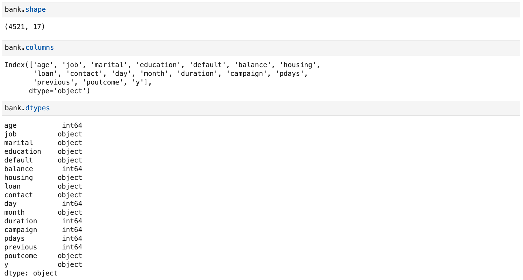
Shape, Columns, and Data Types
-
Use the
shapeattribute to get the shape of aDataFrameor aSeries -
DataFrame→ tuple(row_count, column_count) -
Series→ singleton tuple(length, ) -
The column names of a
DataFramecan be accessed using itscolumnsattribute -
Use the
dtypesattribute to check the data types of aSeriesor aDataFrame's columns -
pandas mostly relies on NumPy arrays and dtypes (
bool,int,float,datetime64[ns], ...) -
pandas also extends some NumPy types (
CategoricalDtype,DatetimeTZDtype, ...) -
Two ways to represent strings:
objectdtype (default) orStringDtype(recommended)
Shape, Columns, and Data Types
Technical Summary
-
A technical summary of a
DataFramecan be accessed using theinfo()method
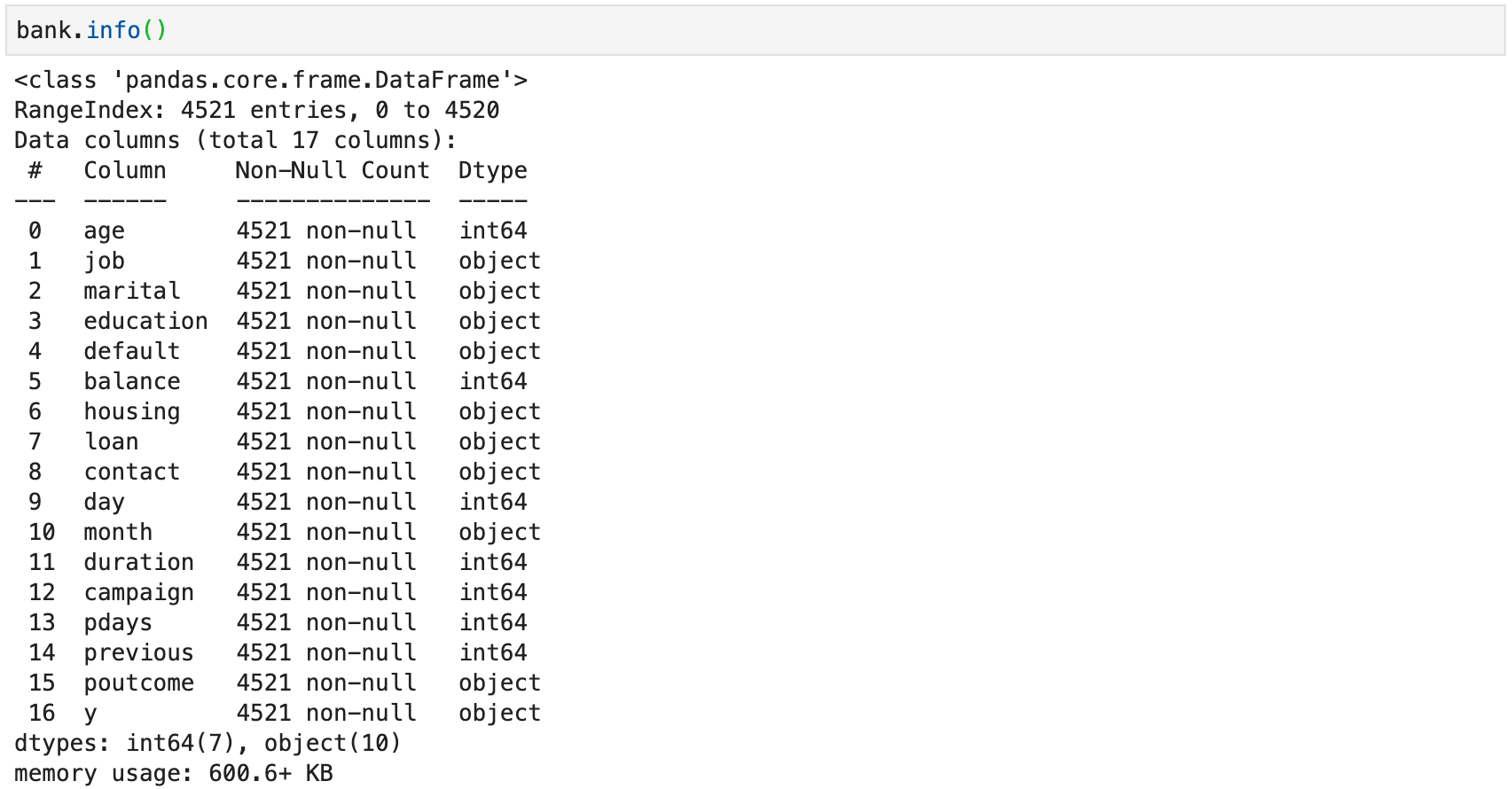
Technical Summary
- The technical summary contains
- The type of the
DataFrame -
The row index (
RangeIndexin the example) and its number of entries - The total number of columns
- For each column
- The column's name
- The count of non-null values
- The column's data type
- Column count per data type
- Total memory usage
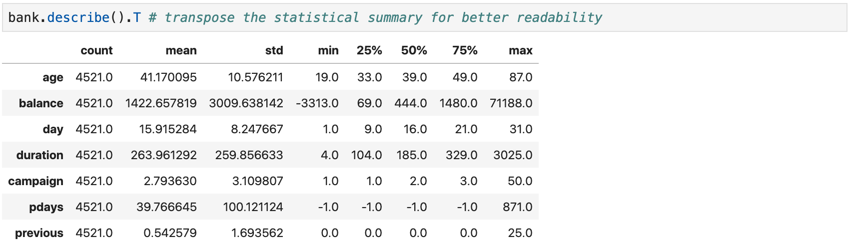
Statistical Summary of Numerical Columns
-
Use the
describe()method to access a statistical summary (mean, standard deviation, min, max, ...) of numerical columns of aDataFrame
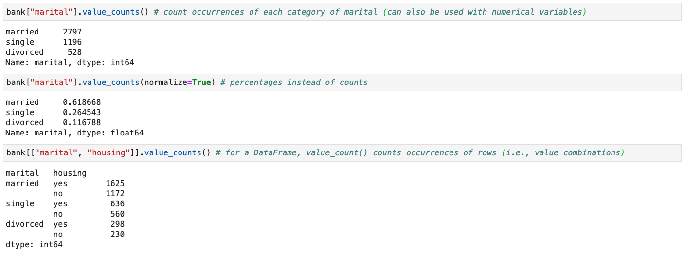
Value Counts of Qualitative Columns
-
Use the
value_counts()method to count the number of occurrences of each value in aSeries(orDataFrame) -
Use
normalize=Truein the method call to get percentages
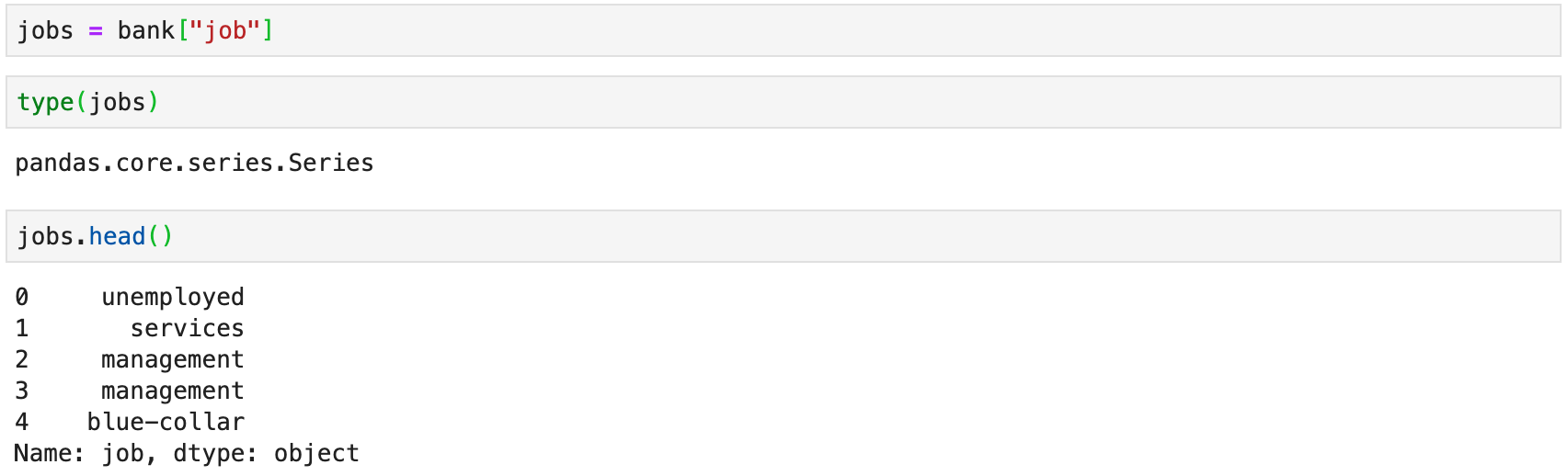
Selecting a Single Column
-
To select a single column from a
DataFrame, specify its name within square brackets →df[col] - The retrieved object is a
Series
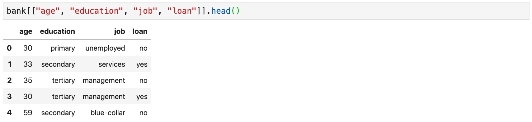
Selecting Multiple Columns
-
To select multiple columns, provide a list of column names within square
brackets →
df[[col_1, col_2, ...]] - The retrieved object is a
DataFrame
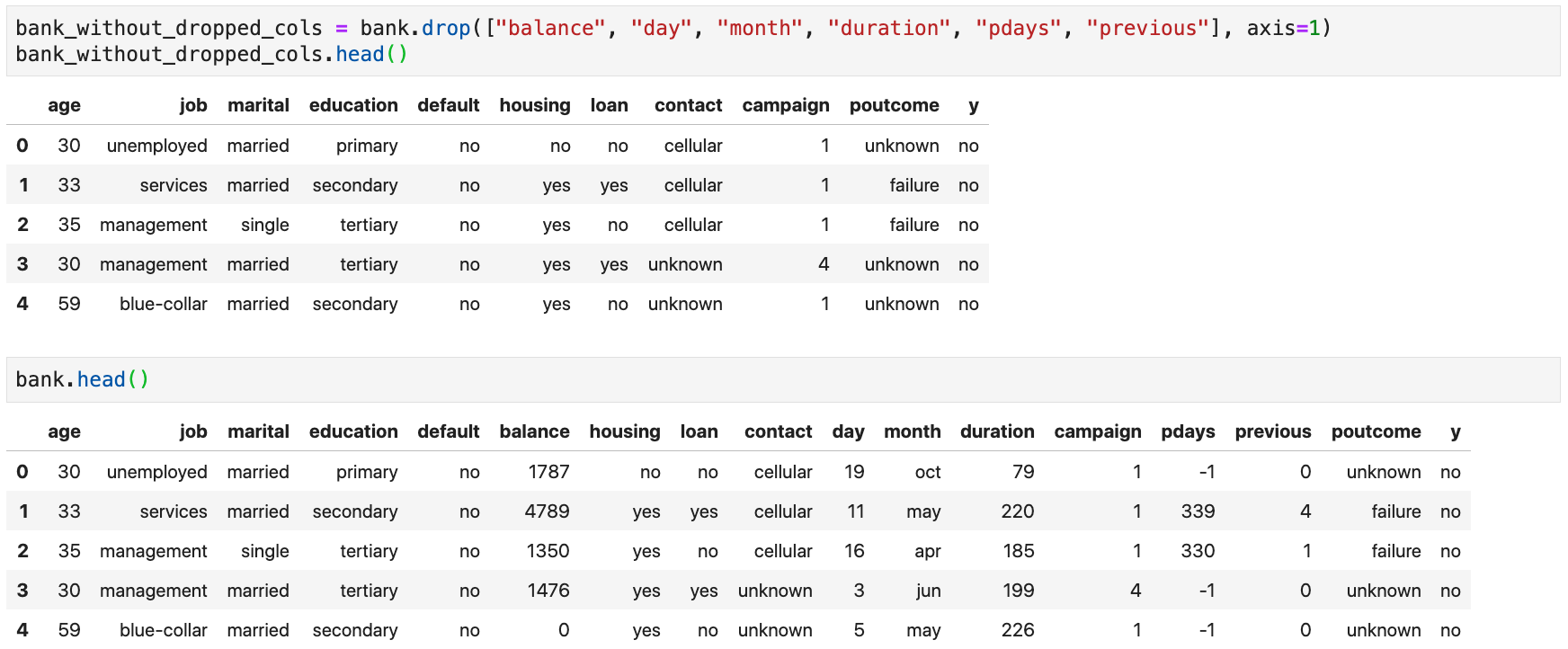
Dropping Columns
-
Instead of selecting columns, you can drop unwanted columns using the
drop()method -
Be sure to specify
axis=1(otherwise, will attempt to drop rows) -
To modify the original data frame, use
inplace=Truein the method call
Why Select Columns?
- Two main motivations for selecting or dropping columns
- Restrict the data to meaningful variables that are useful for the intended data analysis
- Retaining variables that are compatible with some technique you intend to use
- e.g., some machine learning algorithms only make sense when applied to numerical variables
Filtering Rows
-
Rows can be removed using a boolean filter →
df[bool_filter] -
Filter contains
Trueat positioni→ keep corresponding row -
Filter contains
Falseat positioni→ remove corresponding row - Most of the time, the filter involves conditions on the columns
- e.g., keep married clients only
- e.g., keep clients who are 30 or older
- etc.
- Conditions can be combined using logical operators
&→ bit-wise logical and (binary)|→ bit-wise logical or (binary)~→ bit-wise logical negation (unary)
Filtering Rows
- Example: clients who are married or divorced, unemployed, and 40 or older
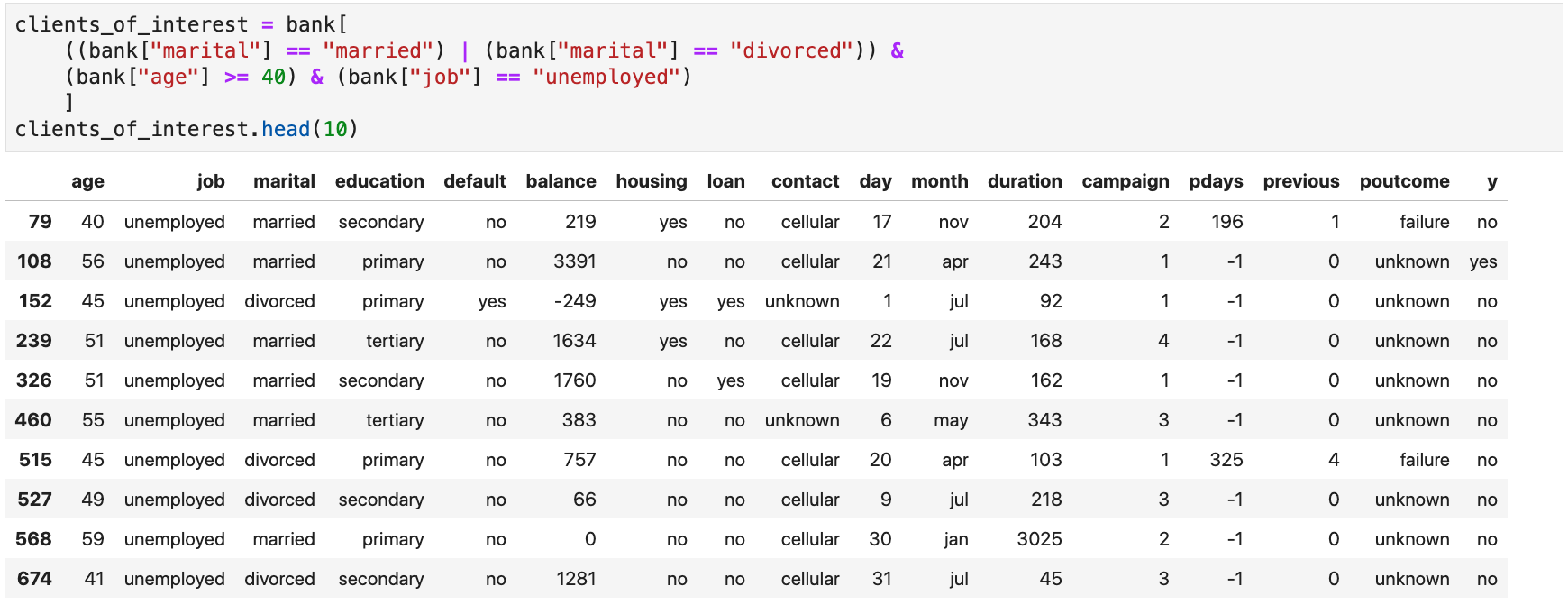
Each condition produces a pandas
Series. The different conditions' Series are then
combined into one Series used to filter the rows.
Why Filter Rows?
- Filtering rows can be motivated by multiple reasons
- Limiting the analysis to a specific subpopulation of interest
- Handling outliers and missing values (drop problematic rows)
- Performance considerations (subsampling a massive data set)
Never filter rows (or select
columns) using
for loops!
Sorting Data
-
Use the
sort_values()method to sort aDataFrameor aSeries - Data frames can be sorted on multiple columns by providing the list of column names
-
Sorting order (ascending or descending) can be controlled with the
ascendingargument -
Use
inplace=Truein the method call to modify the originalDataFrameorSeries
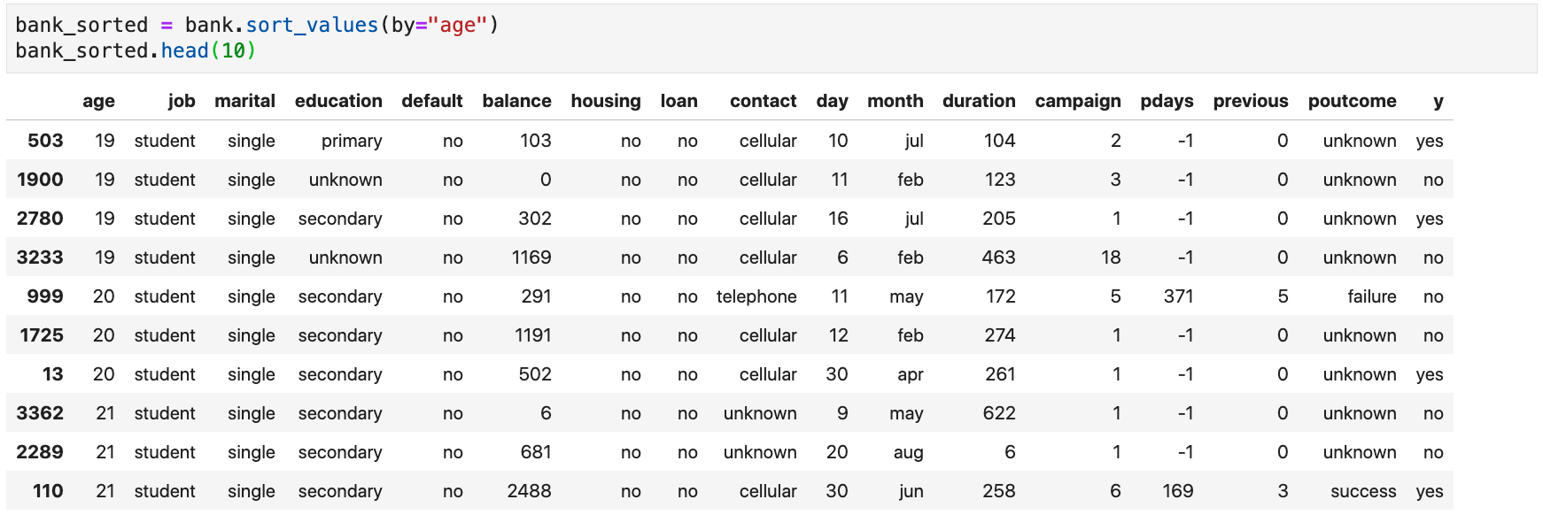
Sorting Data
- Example: sort the data frame by increasing order of age
Sorting Data
- Example: sort the data frame by decreasing alphabetical order of marital status and education, and increasing order of age
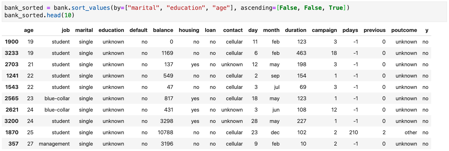
While
education is
an ordinal variable, pandas sorts it alphabetically since it is encoded as a
string!
Indexing Rows and Columns
Indexing Rows and Columns
Two main ways for indexing data frames
- Label-based indexing with
.loc
df.loc[row_lab_index, col_lab_index]- A label-based index can be
- A single label (e.g.,
"age") -
A list or array of labels (e.g.,
["age", "job", "loan"]) - A slice with labels (e.g.,
"age":"balance") - A boolean array or list
.ilocdf.iloc[row_pos_index, col_pos_index]- Similar to NumPy arrays indexing
- A position-based index can be
- An integer (e.g.,
4) - A list or array of integers (e.g.,
[4, 2, 10]) - A slice with integers (e.g.,
2:10:2) - A boolean array or list
:)
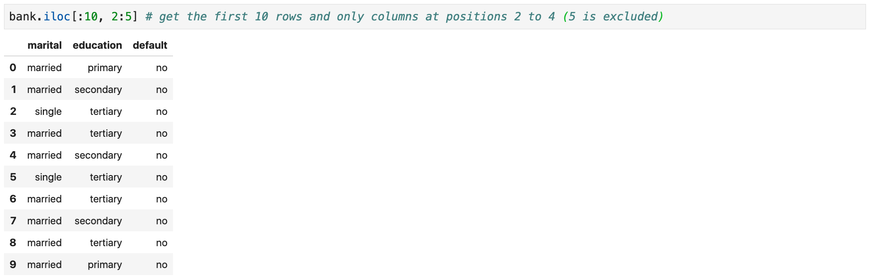
Position-Based Indexing
- Using
.ilocto get rows and columns by position
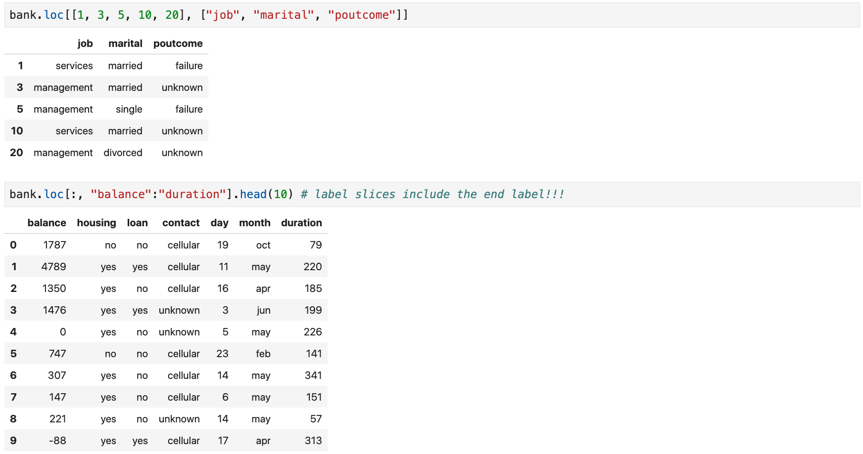
Label-Based Indexing
- Using
.locto get rows and columns by label
Modifying a DataFrame's Row Index
-
A
DataFrame's row index can be changed using theset_index()method -
Use
inplace=Truein the method call to modify the originalDataFrame - The new index can be
- One or more existing columns (provide the list of names)
- One or more arrays, serving as the new index (less common)
- The new index can replace the existing one or expand it
-
The ability to modify the
DataFrame's index enables more interesting label-based indexing of the rows
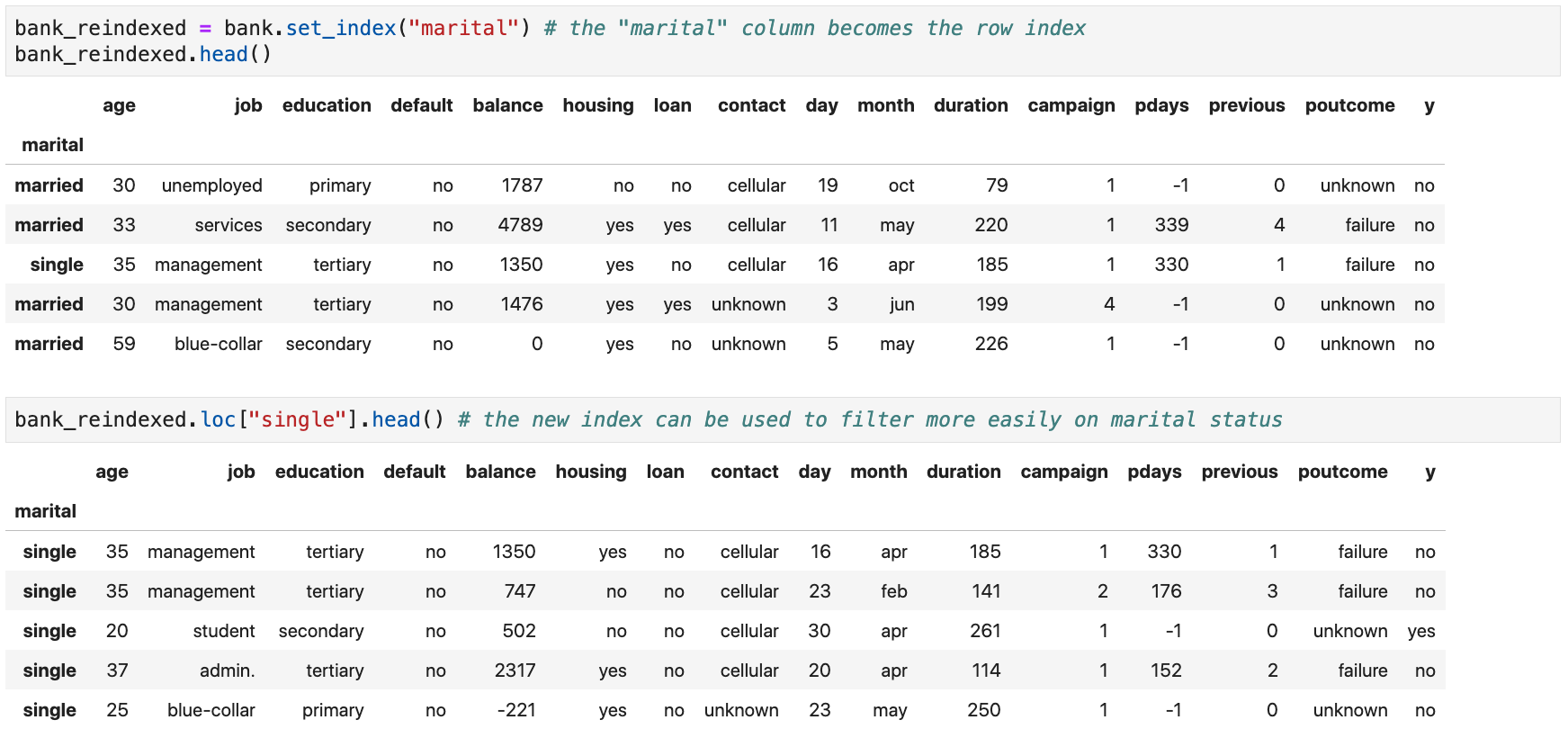
Modifying a DataFrame's Row Index
-
Example: use the
maritalcolumn as theDataFrame's row index (instead of the defaultRangeIndex)
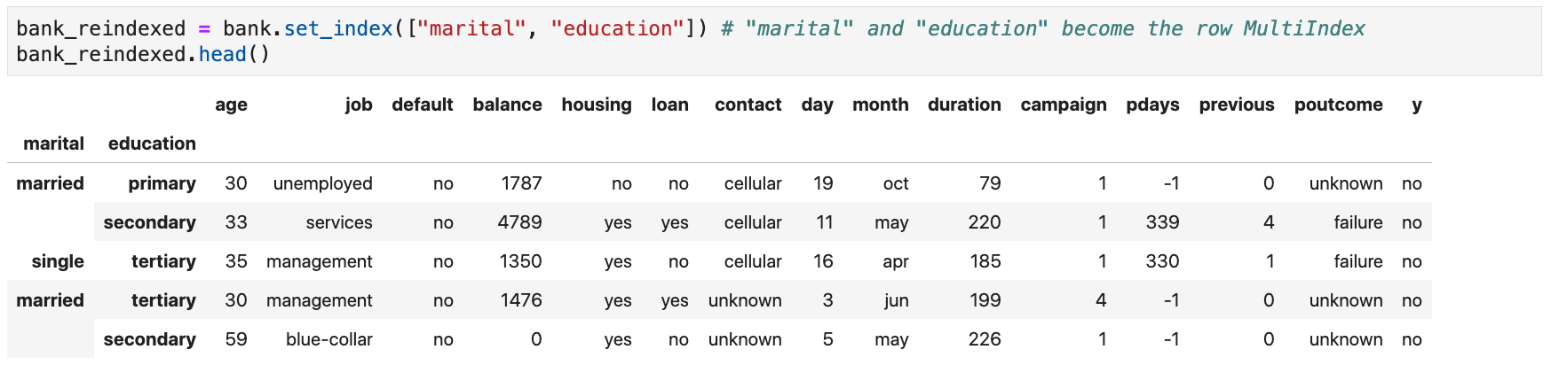
Modifying a DataFrame's Row Index
- Multiple columns can be used as the (multi-level) row index
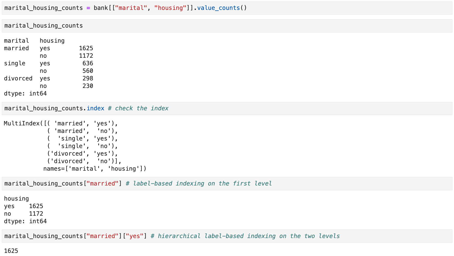
Hierarchical Indexing (MultiIndex)
-
A pandas
DataFrameorSeriescan have a multi-level (hierarchical) index
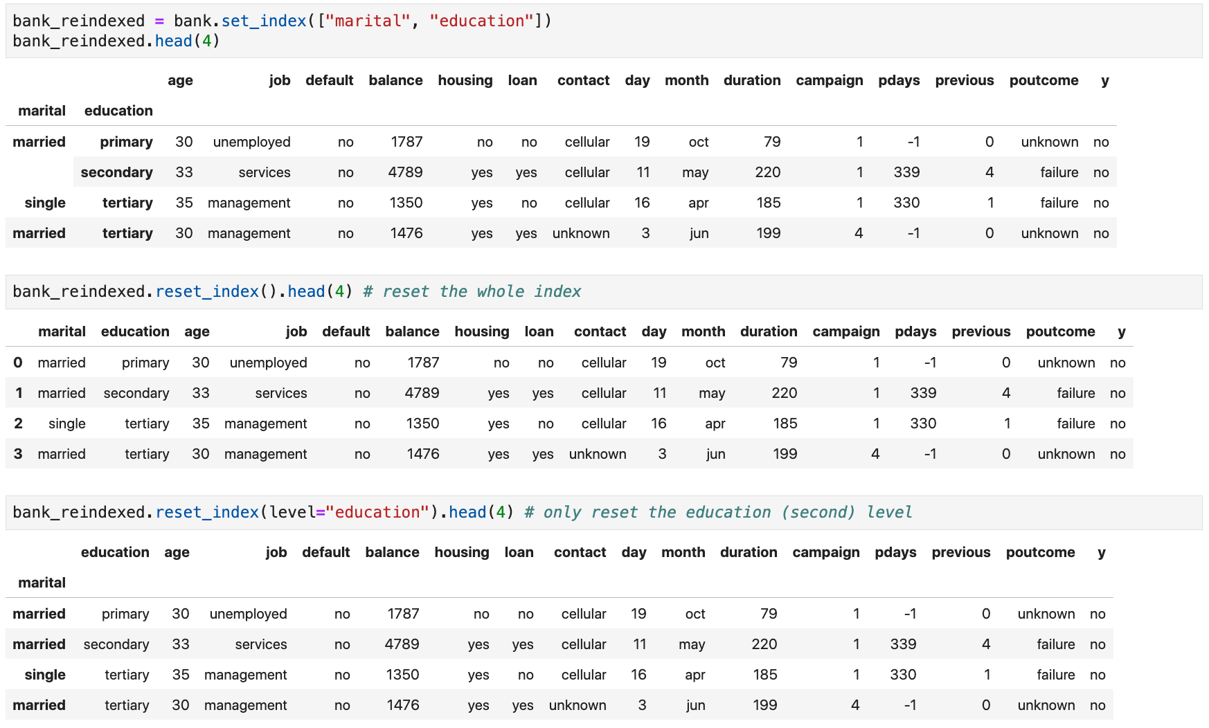
Resetting a DataFrame's Index
-
You can
reset the
DataFrame's index to the default one by using thereset_index()method -
By default, pandas will re-insert the index as columns in the dataset
(use
drop=Truein the method call to drop it instead) -
Use
inplace=Truein the method call to modify the originalDataFramedirectly -
For a
MultiIndex, you can select which levels to reset (levelparameter)
Resetting a DataFrame's Index
Working with Variables
Data Cleaning
- Toy data sets are clean and tidy
- Real data sets are messy and dirty
- Duplicates
- Missing values
- e.g., a sensor was offline or broken, a person didn't answer a question in a survey, ...
- Outliers
- e.g., extreme amounts, ...
- Value errors
- e.g., negative ages, birthdates in the future, ...
- Inconsistent category encoding and spelling mistakes
-
e.g.,
"unemployed","Unemployed","Unemployd", ... - Inconsistent formats
-
e.g.,
2020-11-19,2020/11/12,2020-19-11, ... - If nothing is done → garbage in, garbage out!!! 💩💩💩
Deduplicating Data
-
Use the
duplicated()method to identify duplicated rows in aDataFrame(or values in aSeries) -
Use
drop_duplicates()to remove duplicates from aDataFrameorSeries -
Use
inplace=Trueto modify the originalDataFrameorSeries -
Use the
subsetargument to limit the columns on which to search for duplicates -
Use the
keepargument to indicate what item of the duplicates must be retained (first, last, drop all duplicates)
Deduplicating Data
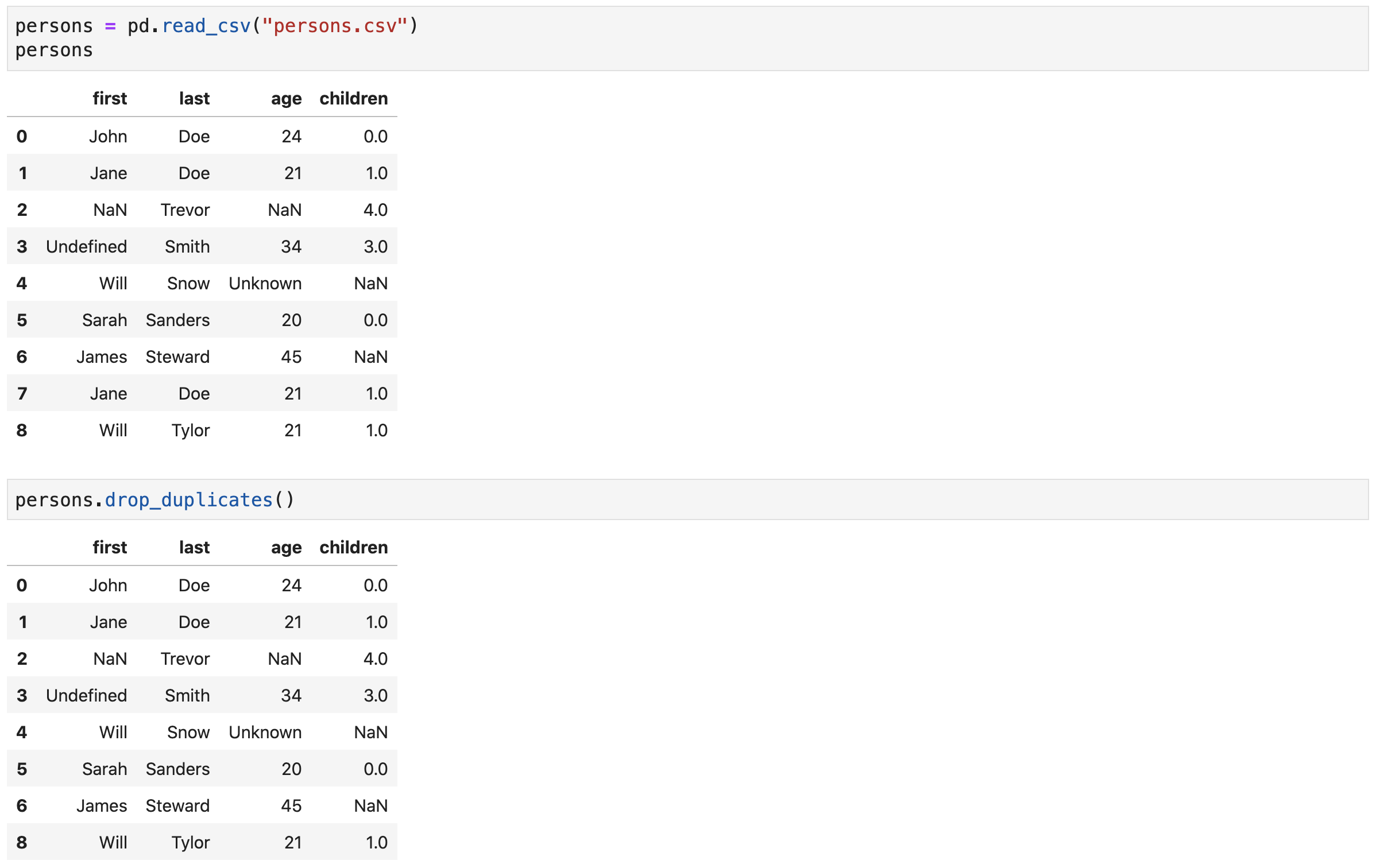
Download
persons.csv
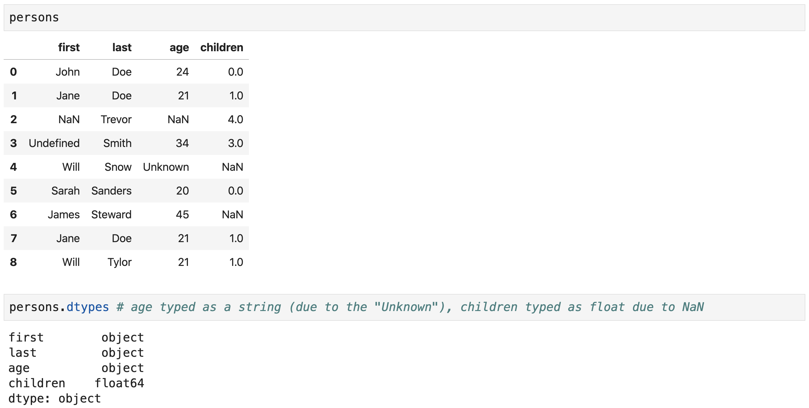
Dealing with Missing Values
- Two main strategies for dealing with missing values
- Remove rows (or columns) with missing values → viable when the data set is big (or if impacted columns are not important)
- Replace the missing values
- Using basic strategies (e.g., replace with a constant, replace with the column's median, ...)
- Using advanced strategies (e.g., ML algorithms that infer missing values based on values of other columns)
Dealing with Missing Values
The presence of missing values
can have serious repercussions on the column data types!
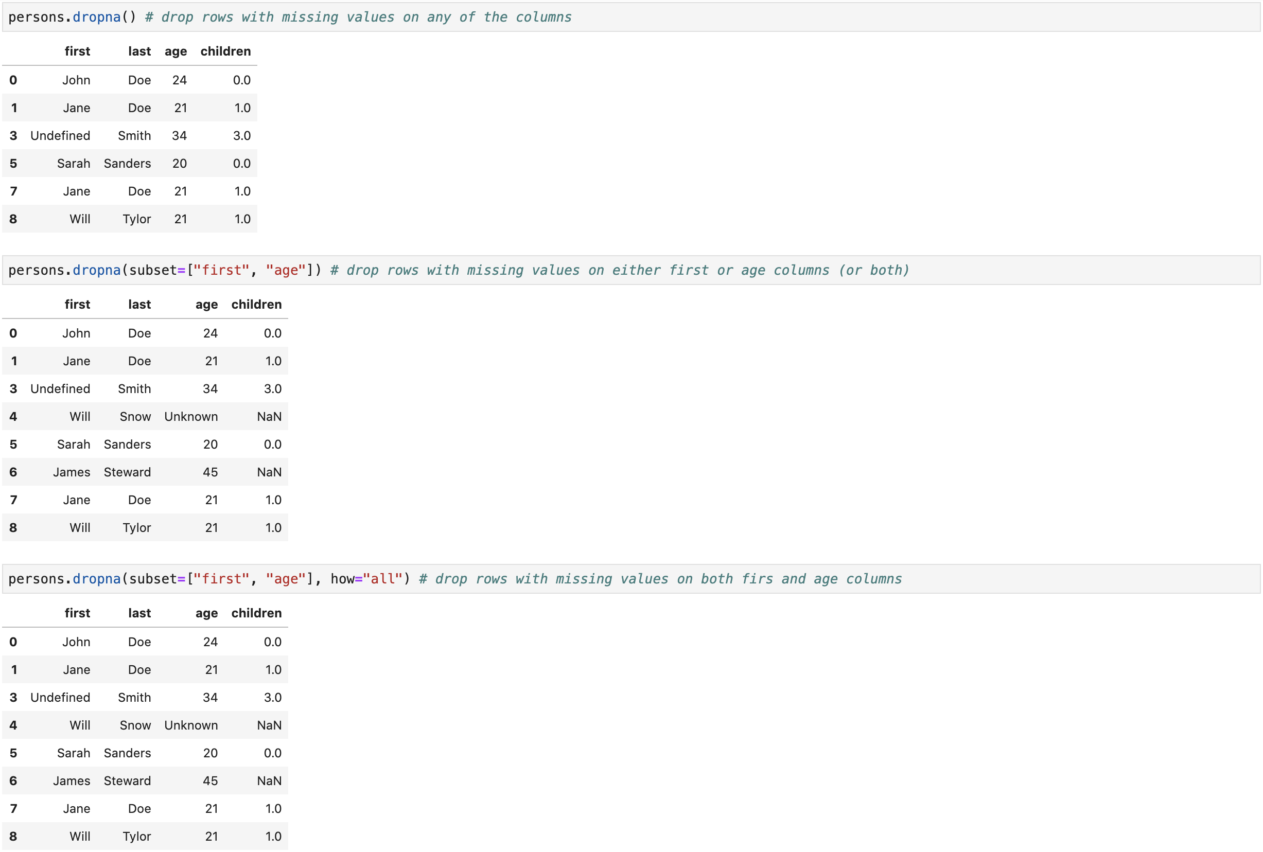
Dropping Missing Values
-
Use the
dropna()method to remove rows (or columns) with missing values - Important arguments
-
axis: axis along which missing values will be removed -
how: whether to remove a row or column if all values are missing ("all") or if any value is missing ("any") -
subset: labels on other axis to consider when looking for missing values -
inplace: ifTrue, do the operation on the original object
Dropping Missing Values
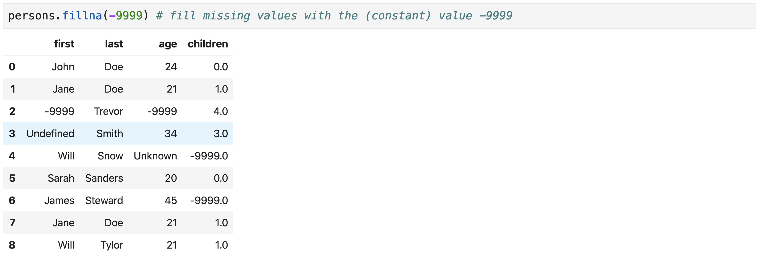
Replacing Missing Values
-
Use the
fillna()method to replace missing values in aDataFrame - Important arguments
value: replacement valueaxis: axis along which to fill missing values-
inplace: ifTrue, do the operation on the originalDataFrame
Replacing Missing Values
Recasting Variables
- Variables should be typed with the most appropriate data type
-
Binary variables should be encoded as booleans or
0,1 - Discrete quantitative variables should be encoded as integers
- Depending on the intended goal, categorical features can be dummy-encoded
- etc.
-
Use the
convert_dtypes()method to let pandas attempt to infer the most appropriate data types for a data frame's columns -
Use the
astype()method to recast columns (Series) to other types
The most appropriate data type is
often task-dependant!
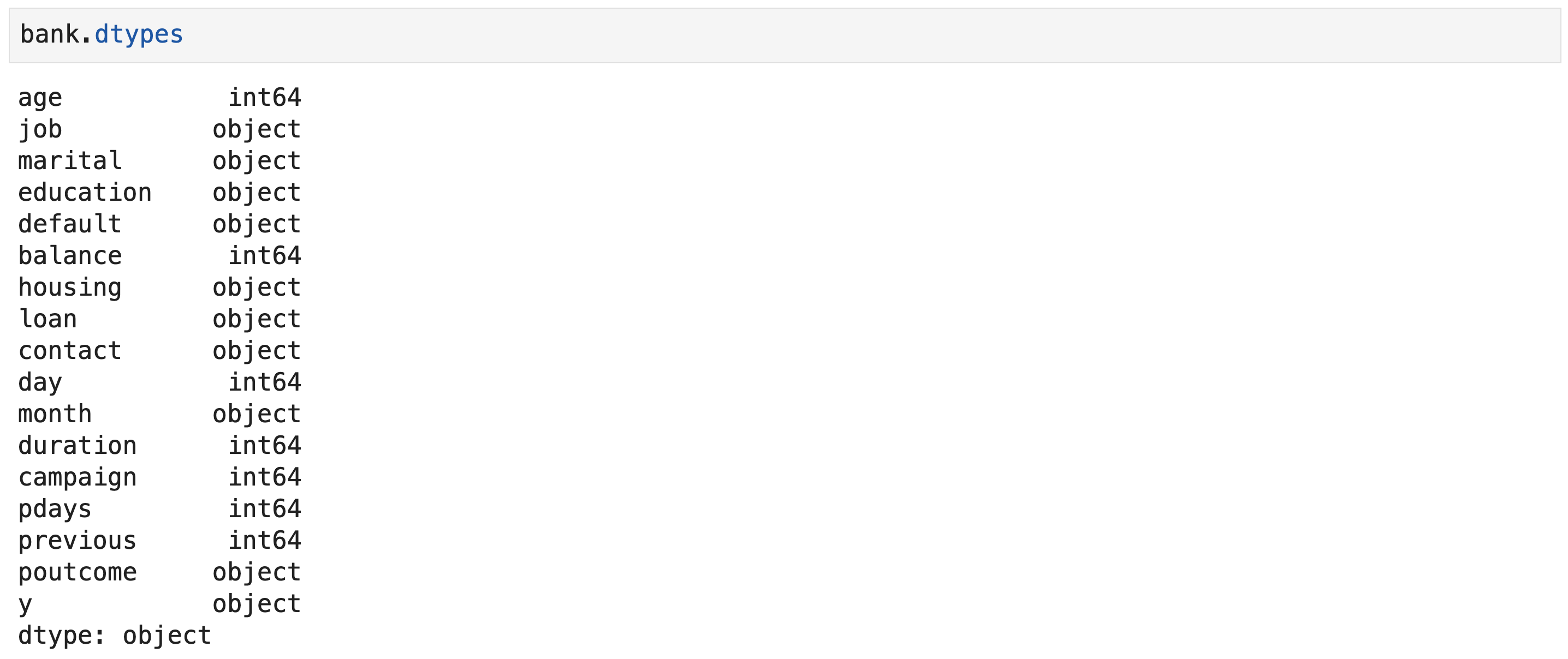
Recasting Variables
- Original data types in the bank data frame
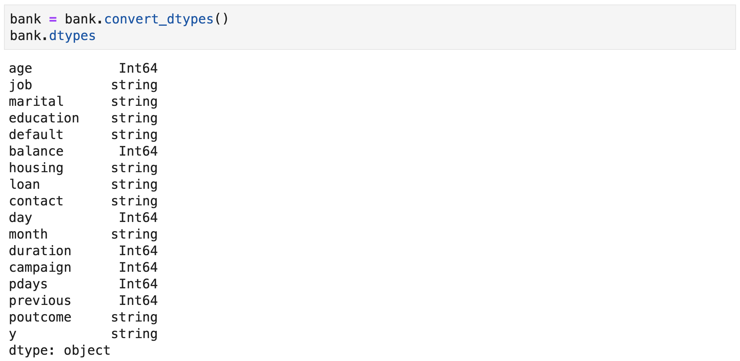
Recasting Variables
- Data types after using the
convert_dtypes()method
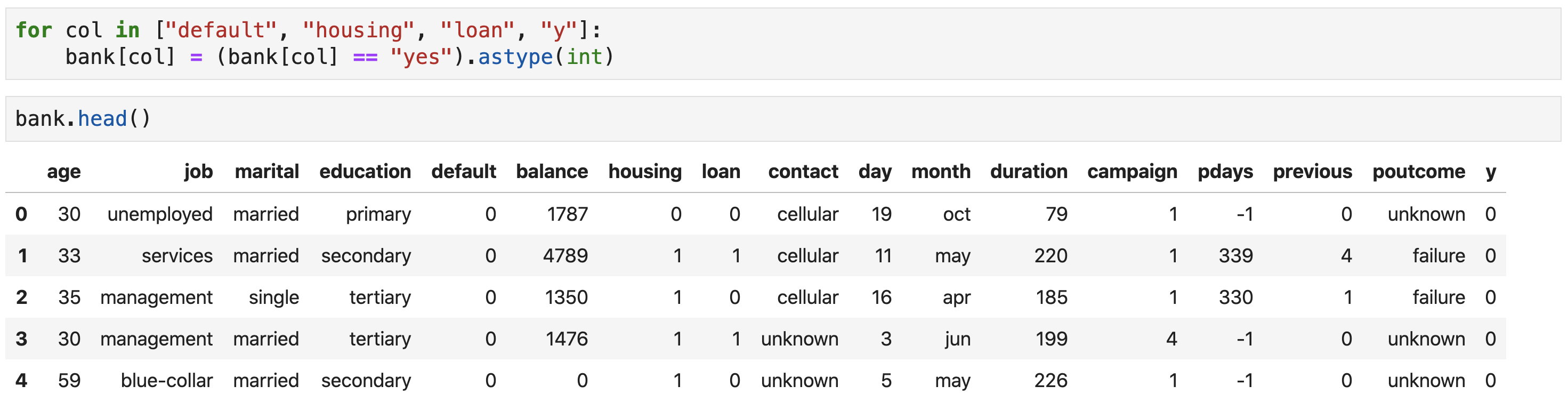
Recasting Variables
- Converting binary (yes/no) variables to 0, 1
Recasting Variables
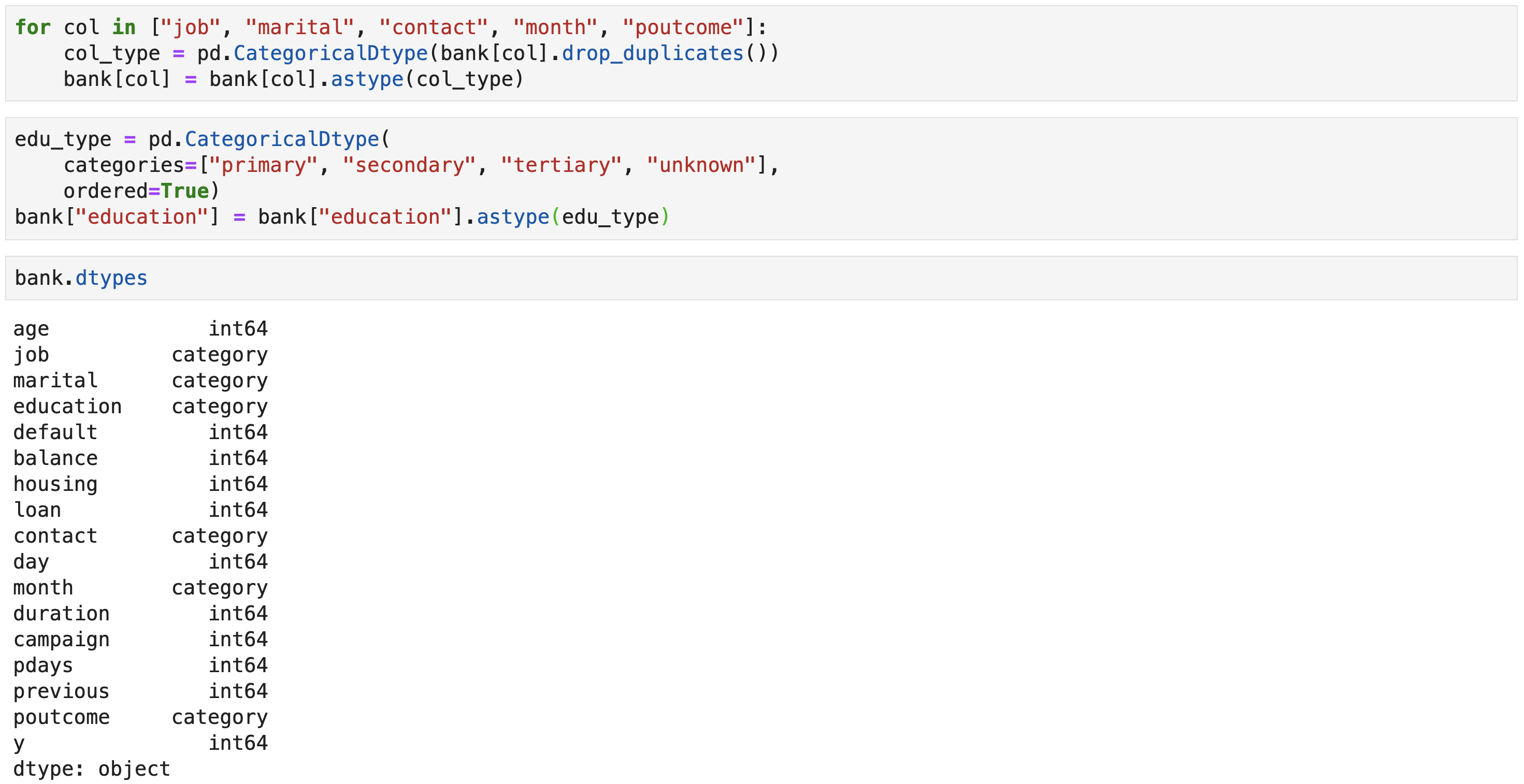
-
Recasting categorical variables from strings to pandas'
CategoricalDtype
Recasting Variables
- Sorting on
educationrespects the category order now
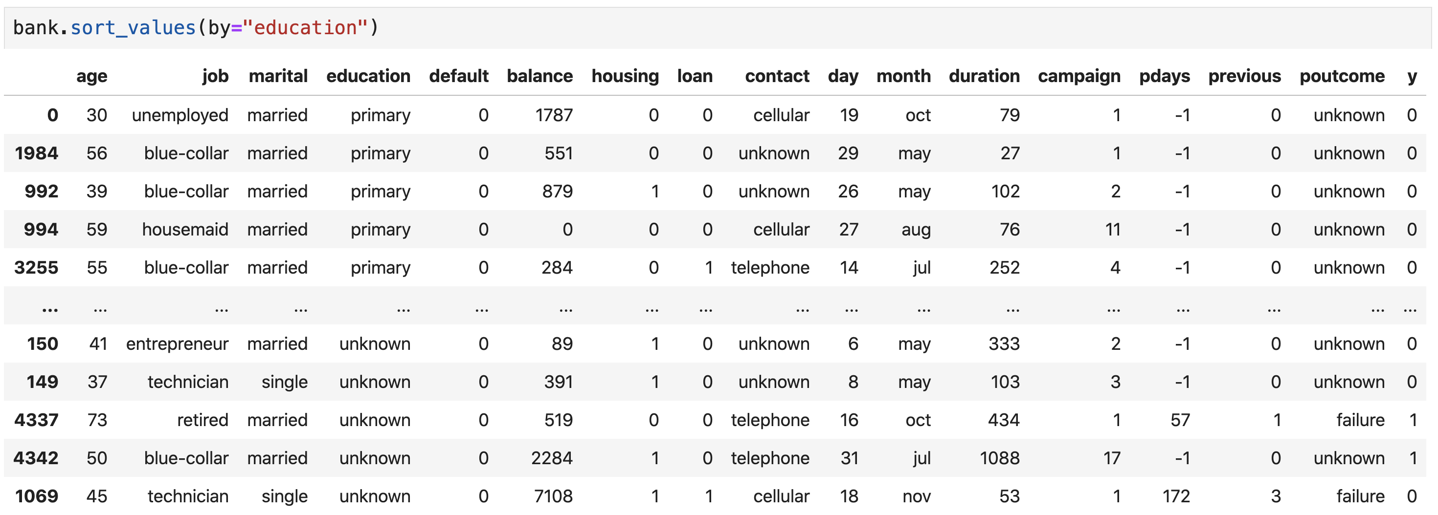
In practice, categorical variables are
often left as strings and not encoded as
CategoricalDtype.
Creating New Features
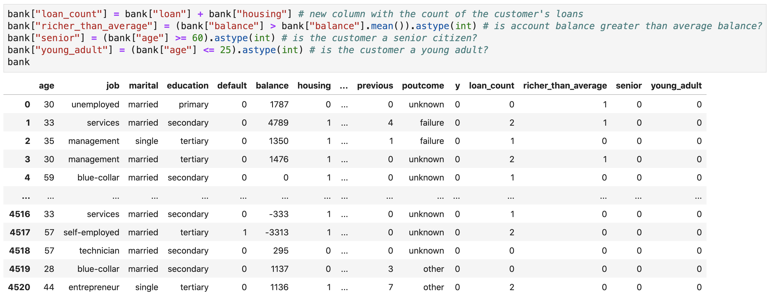
- Data analyses and machine learning often involve feature engineering, i.e., creating new features from existing ones based on domain knowledge (and intuition)
- Examples of feature engineering
- Extracting day of week, month, year, etc. from datetime variables
- Reverse geocoding (i.e., creating country, state, department, etc. fields from geographical coordinates)
- Binning
- One-hot encoding
- Log-transformation
- etc.
Creating New Features
One-Hot Encoding
- Machine learning tasks often require one-hot encoding of categorical variables
- The variable is transformed into multiple columns
- Each column represents a category of the variable
-
A
1on a column indicates which category the original variable had - All the other categories' columns contain
0 -
Use the
get_dummies()function to one-hot encode categorical columns
One-Hot Encoding
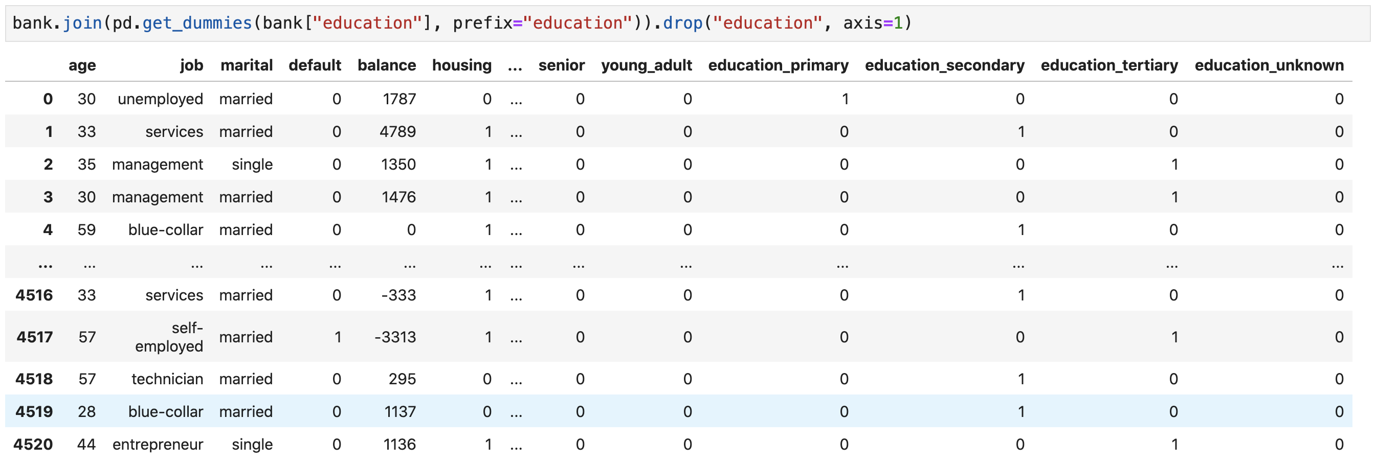
-
Dummy encode the
educationvariable, join the dummy variables to the data frame (more on joins later), and drop the original column
Grouping and Aggregating Data
Group By
- Group by refers to a 3-step process
- Splitting the data into groups based on some criteria (e.g., by marital status)
- Applying a function to each group separately
- Aggregation (e.g., computing summary statistics)
- Transformation (e.g., standardization, NA filling, ...)
- Filtering (e.g., remove groups with few rows or based on group aggregates, ...)
-
Combining the results into a data structure (a
DataFramemost of the time)
If this sounds familiar to you, it is
because this is how
value_counts() works.
Group By

Refer to
the documentation
for details on
DataFrameGroupBy objects and possible
aggregations and transformations.
Group By
- Example: group by marital status and calculate the min, median, and max balance as well as the median age for each group
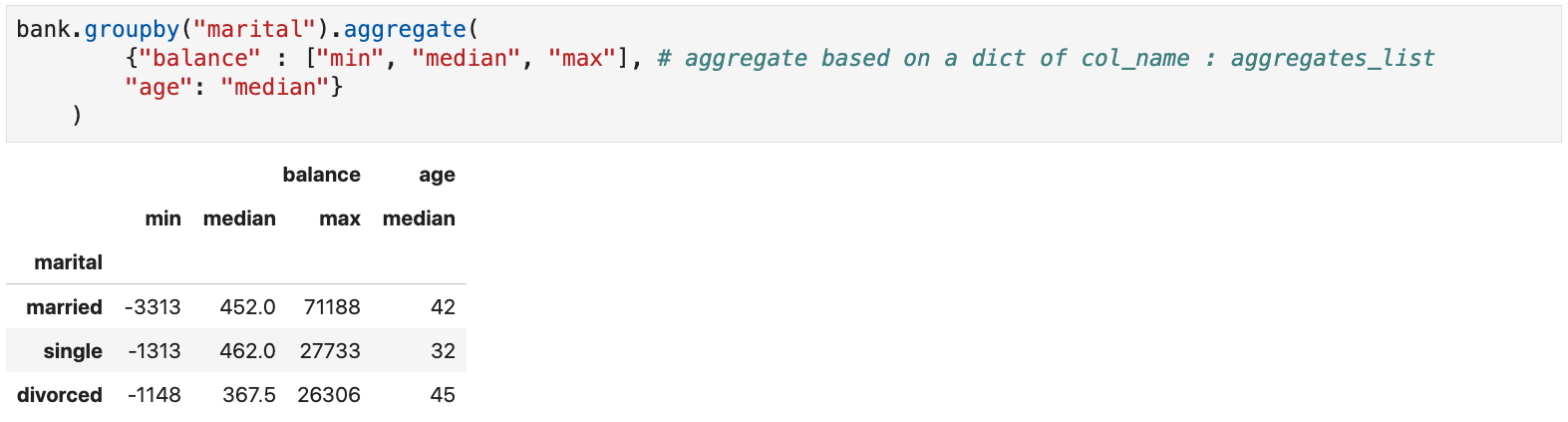
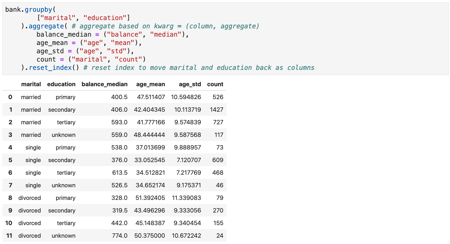
Group By
- Example: group by marital status and education level, then calculate median balance, age mean and standard deviation, and number of rows in each group
Reshaping Data Frames
Pivoting
- Pivoting is useful when studying how a given (numeric) variable is conditioned by two or more (discrete) variables
- The conditioning variables' values are used as dimensions (row and column indexes)
- The cells contain the values of the conditioned variable for the corresponding dimensions

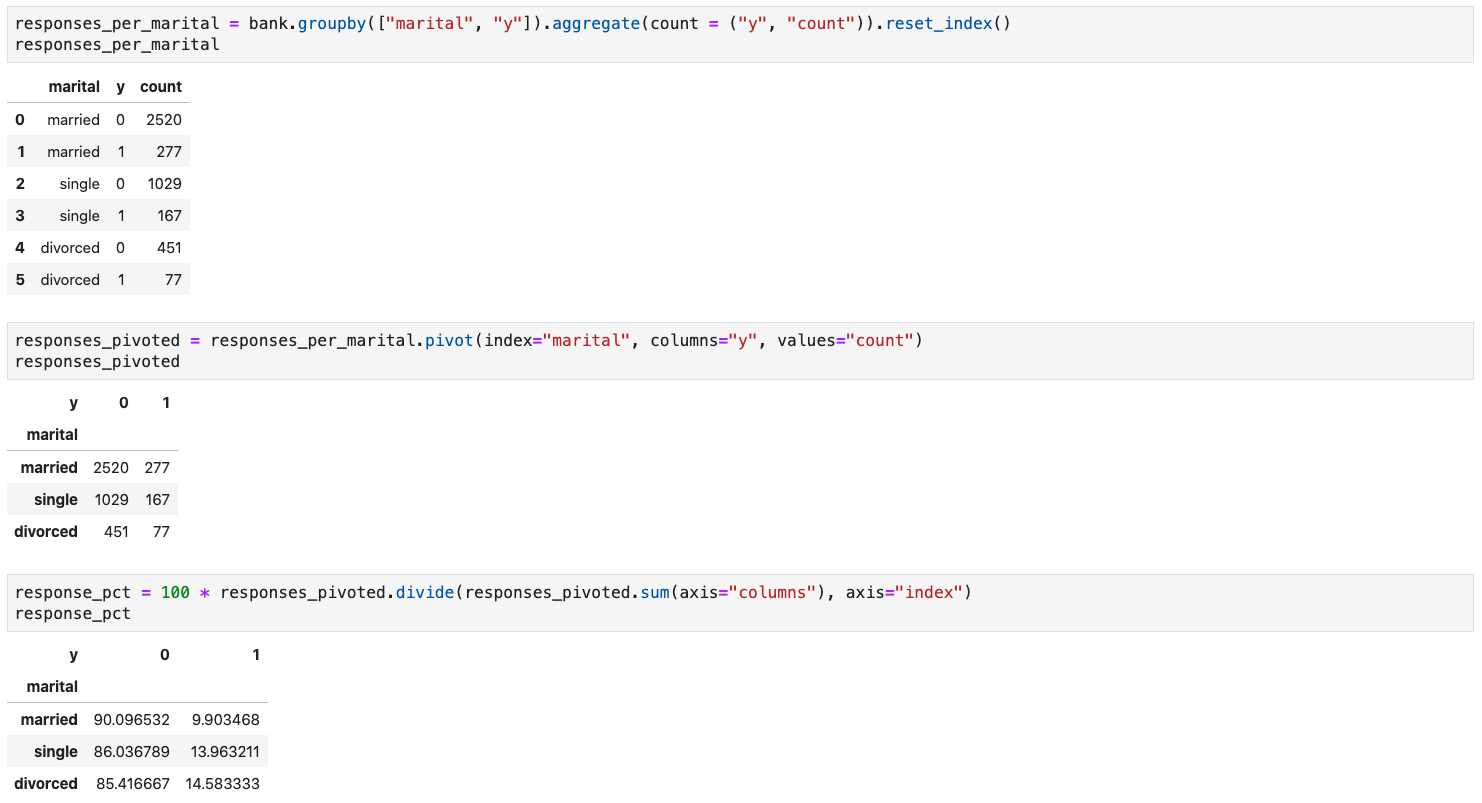
Pivoting
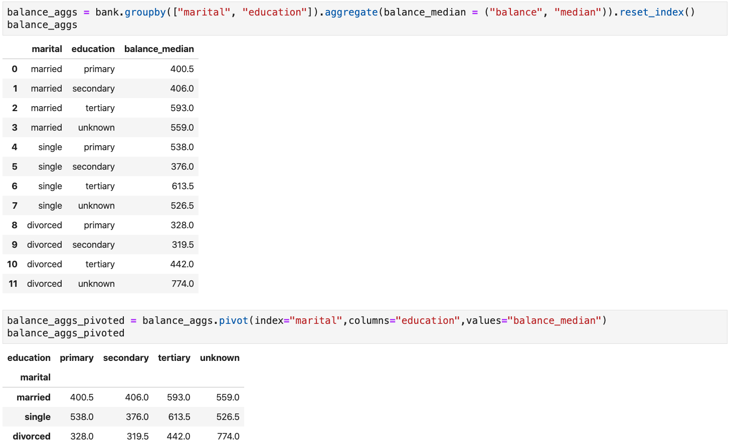
Pivoting
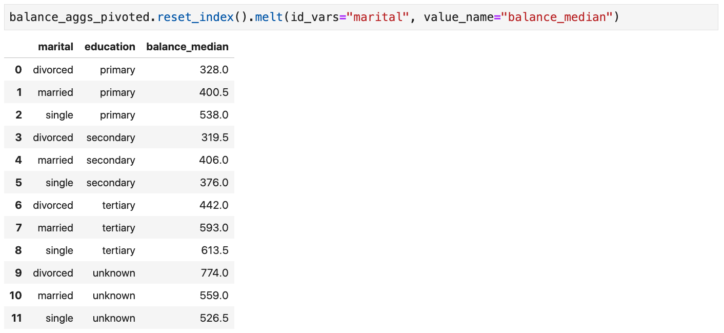
Melting
- Melting can be seen as the inverse of pivoting

Melting
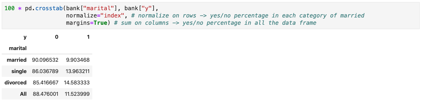
Cross Tabulations
-
Use the
crosstab()function to compute cross tabulations (i.e., co-occurrence counts) of two or more categoricalSeries -
Can be normalized on rows, columns, etc. using the
normalizeargument -
Can be marginalized by passing
margins=Truein the function call
Other Reshaping Operations
- Other reshaping operations include
- Stacking and unstacking
- Pivot tables (generalization of the simple pivot)
- Exploding list-like columns
- etc.
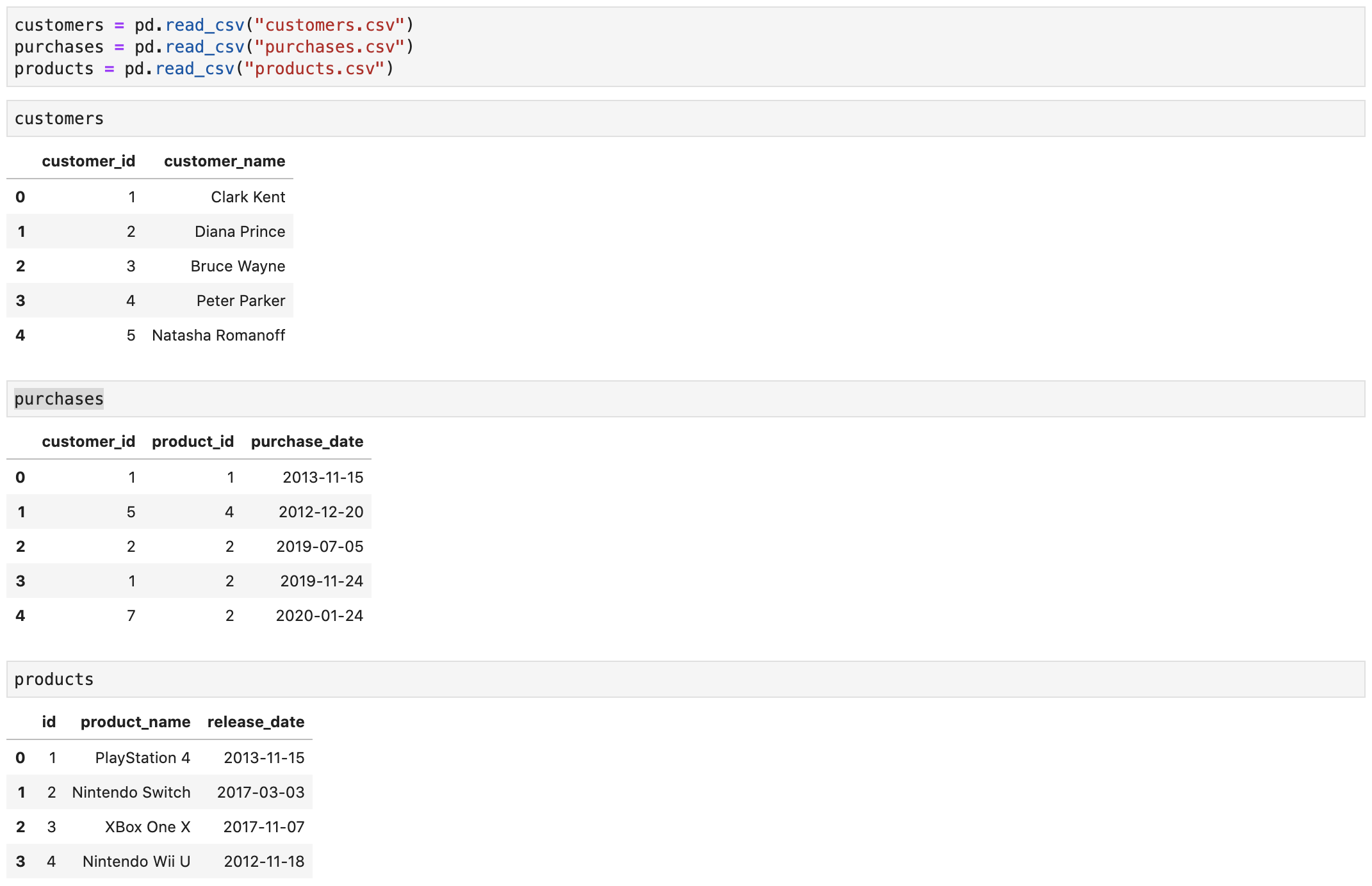
Working with Multiple Tables
Working with Multiple Tables
- Real data sets are often organized in multiple data tables
- Each table describes one entity type
- e.g., a table describes customers, another table describes products, and a third table describes purchases
- Entities can reference other entities they are related to
- In order to conduct your analysis, you need to “patch” these tables together
 Download data set
Working with Multiple Tables
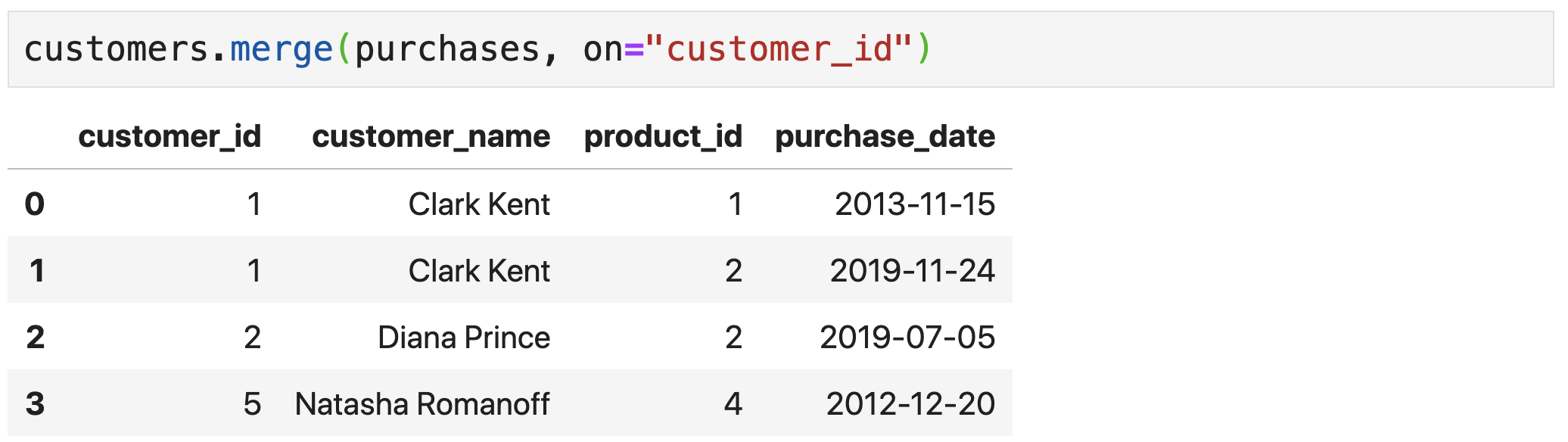
Merging Data Frames
-
Use the
merge()method to merge aDataFramewith anotherDataFrame(orSeries) - The merge is done with a database-style (SQL) join
-
Usually based on one or more common columns (e.g., the
customer_idcolumn in both customers and purchases) - If a row from the left object and a row from the right object have matching values for the join columns → a row combining the two is produced
- If no match is found → output depends on the join type
- Inner join → no row is produced
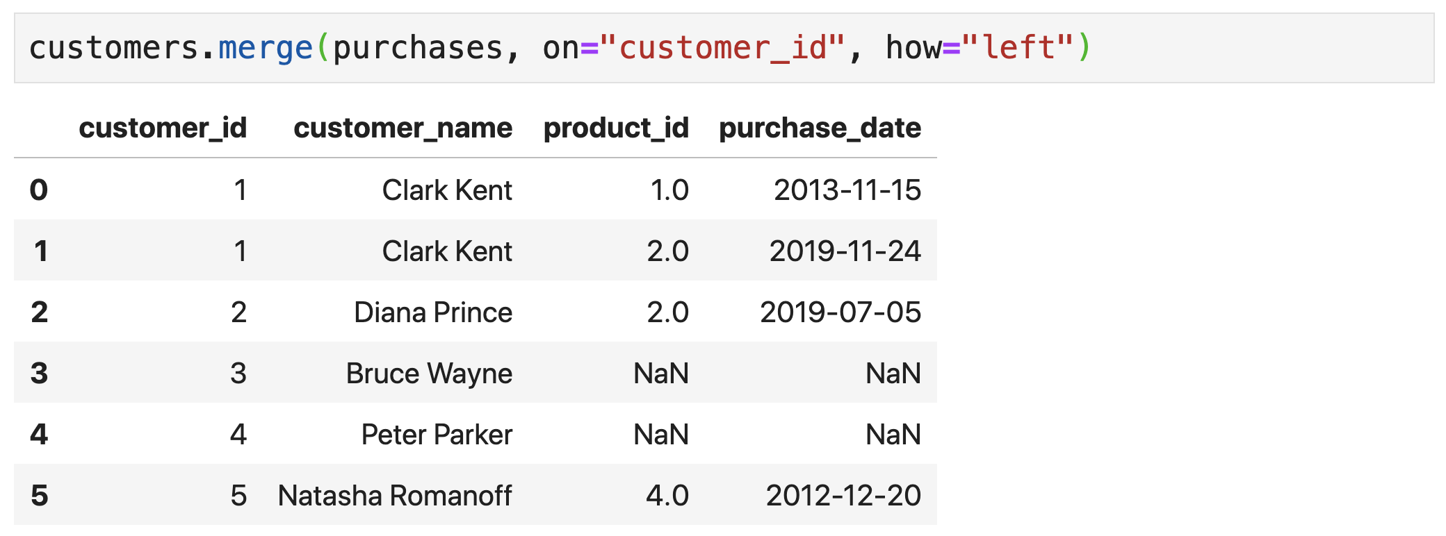
- Left join → for left rows with no match, produce a row (with NA filled right row)
- Right join → for right rows with no match, produce a row (with NA filled left row)
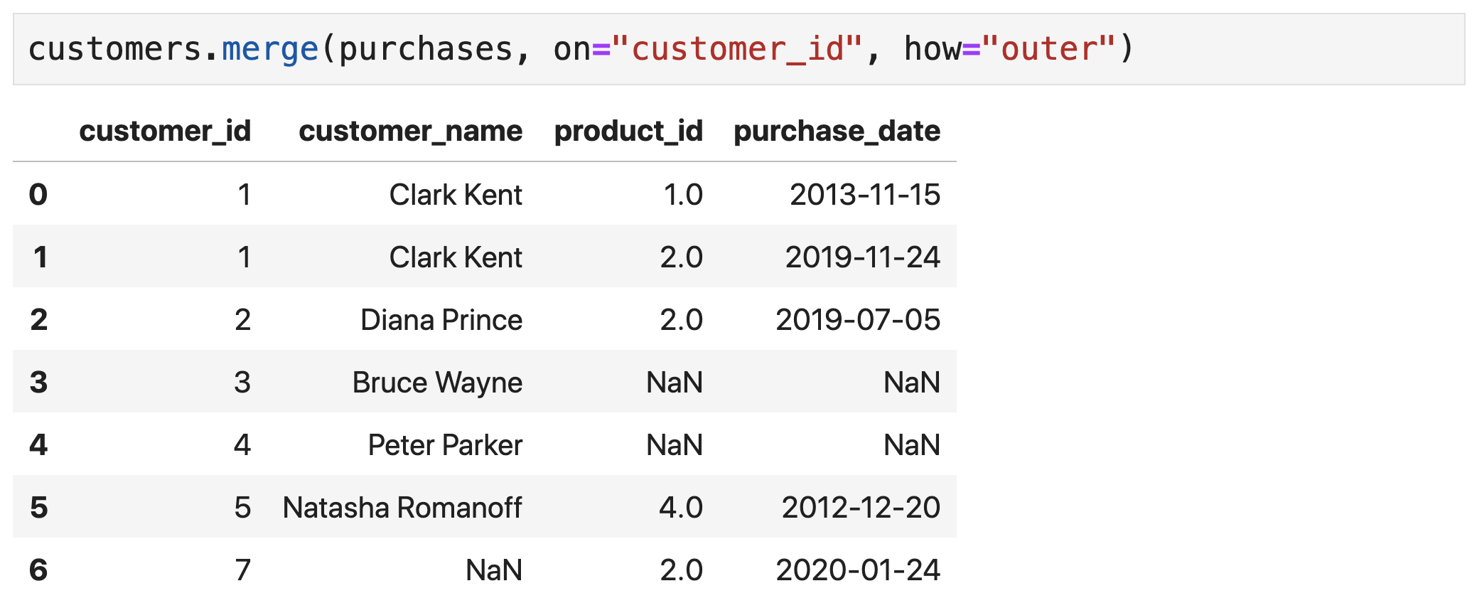
- Outer join → combination of left and right join
- Joins can also be performed on rows (less common)
Merge Types
Inner Join
Left Join
Right Join

Outer Join
Merging Data Frames
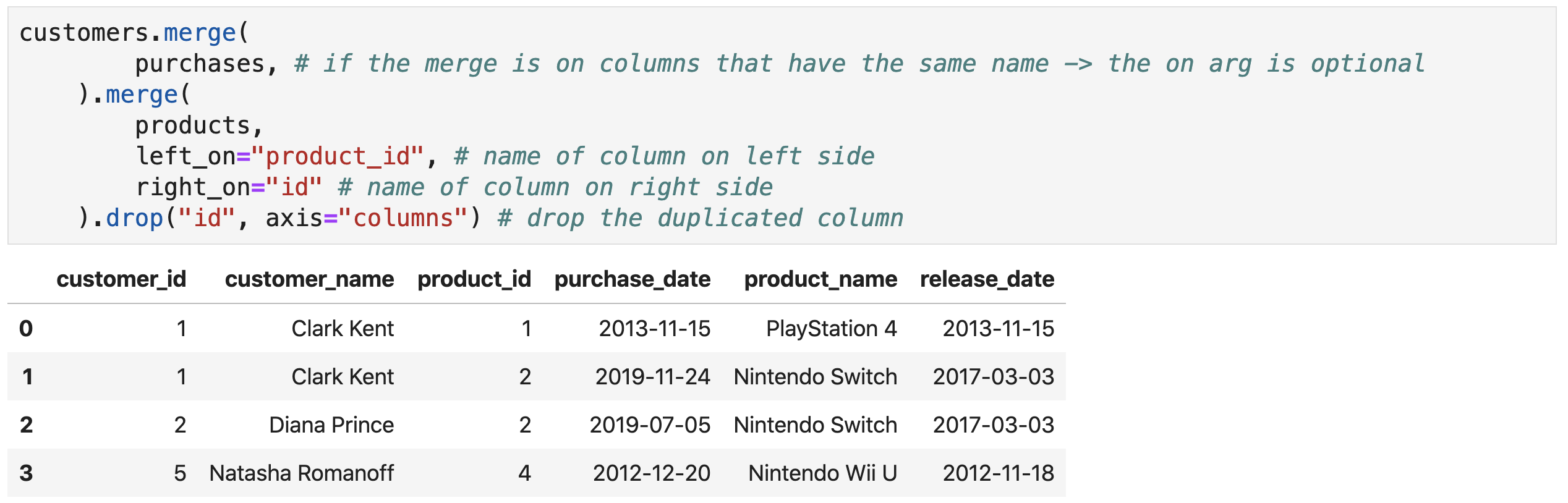
- Multiple tables can be merged together (consecutively)
-
Sometimes, the merge is on columns that do not have the same names (e.g.,
the
idcolumn in products and theproduct_idcolumn in purchases) -
Use the
left_onandright_onarguments to specify the column names in the left and right data frames respectively
Creative Commons
Attribution-NonCommercial-ShareAlike 4.0
International Public License
(CC BY-NC-SA 4.0)
Python for Data Science A Crash Course Processing Tabular Data With pandas Khalil El Mahrsi 2025