Python for Data Science: a Crash Course Scientific Computing With NumPy

Extending Python with Packages

Python's functionalities can be further extended by installing additional packages

From the PyPI (Python Package Index) repository
From Conda channels (useful for optimized package versions)
From source code (often distributed through GitHub repos)

Two main tools for package installation

The package installer for Python (pip)
Conda* (recommended if package available through Conda)

Using conda (recommended)

% conda install package_name

Using pip

% pip install package_name

* Packages can also be installed through Anaconda Navigator (GUI)

Importing Modules

In order to be able to use a module, you first need to import it with an import statement
Three possible ways

Simple import of a whole module

>>> import module_name

Import a module with an alias (i.e., give it a new name)

>>> import module_name as alias

Import specific items from a module

>>> from module_name import item_1, item_2, ...

What is NumPy?

A fundamental Python package for scientific computation
Almost every other Python data science package (pandas, scikit-learn, matplotlib, ...) relies on NumPy
NumPy provides

An object type (the ndarray) for representing multidimensional arrays (vectors, matrices, tensors, ...)
Optimized routines and array operations

Shape manipulation (indexing and slicing, reshaping, ...)
Linear algebra and mathematical operations
Statistics
Random simulation
Discrete Fourier transforms
...

Installing and Importing NumPy

Installing NumPy with conda (recommended)

% conda install numpy

Installing NumPy with pip

% pip install numpy

Importing NumPy (in Python scripts or notebooks)

>>> import numpy as np

A Simple One-Dimensional NumPy Array

>>> import numpy as np # import NumPy under the alias np
>>> np.__version__ # check version'1.19.1'>>> a = np.array([0, 1, 2, 3, 4]) # create array from a list
>>> print(a)[0 1 2 3 4]>>> type(a) # check array type -> ndarray<class 'numpy.ndarray'>>>> print(a[2]) # NumPy arrays are subscriptable3>>> print(a[1::2]) # slicing is also supported[2 4]>>> a[4] = 7 # NumPy arrays are mutable
>>> print(a)[1 2 3 4 7]

Why Not Just Use Lists?

Lists are general-purpose sequences

Efficient when it comes to insertions, deletions, appending, ...
No support for vectorized operations (e.g., element-wise addition or multiplication)
Mixed types → must store type info for every item

NumPy arrays are (way) more efficient

Fixed type (i.e., all elements of an array have the same type)

Less in-memory space
No type checking when iterating

Use contiguous memory → faster access and better caching
Relies on highly-optimized compiled C code
Support of vectorization and broadcasting

NumPy Arrays vs. Lists

>>> import numpy as np
>>> l1, l2 = [0, 1, 2, 3], [4, 5, 6, 7] # two lists
>>> a1, a2 = np.array(l1), np.array(l2) # two NumPy arrays based on those lists
>>> print(l1 + l2) # adding lists results in concatenation[0, 1, 2, 3, 4, 5, 6, 7]>>> print(a1 + a2) # adding NumPy arrays results in element-wise addition[ 4  6  8 10]>>> print(3 * l1) # the * results in list replication...[0, 1, 2, 3, 0, 1, 2, 3, 0, 1, 2, 3]>>> print(3 * a1) # ... but results in element-wise multiplication for ndarrays[0 3 6 9]>>> print(l1 * l2) # trying to multiply lists raises an exception...Traceback (most recent call last):
  File "<stdin>", line 1, in <module>
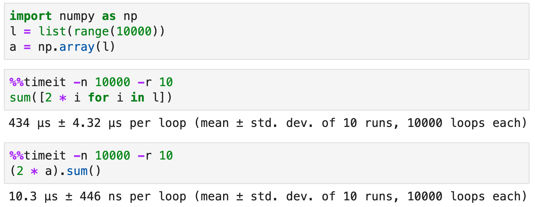
TypeError: can't multiply sequence by non-int of type 'list'>>> print(a1 * a2) # ... but is supported by ndarrays[ 0  5 12 21]

NumPy Arrays vs. Lists

Vectorization, fixed types, compiled C implementations, etc. all contribute to making NumPy significantly faster than built-in Python lists

NumPy Array Basics

>>> import numpy as np
>>> a = np.array([0, 1, 2, 3, 4])
>>> print(a)[0 1 2 3 4]>>> a.ndim # number of dimensions1>>> a.shape # shape (length along each dimension)(5,)>>> a.size # size (total number of items)5>>> a.dtype # dtype (data type)dtype('int64')>>> a.itemsize # item size (in bytes)8>>> a.nbytes # total memory size (in bytes)40>>> a[1] # positional indexing works the same as lists1>>> a[1:4] # same goes for slicingarray([1, 2, 3])>>> a[4] = 12.9 # arrays are mutable but beware of type coercion!array([ 0,  1,  2,  3, 12])

Attributes of interest

shape
ndim
dtype
itemsize
nbytes

Multi-Dimensional Arrays

For the sake of simplification, examples shown here use two-dimensional arrays. The principles remains the same for arrays of higher dimensions.

>>> import numpy as np
>>> # multi-dimensional arrays can be built from lists of lists
>>> a = np.array([
...   [0, 1, 2, 3, 4], # first list -> first row,
...   [5, 6, 7, 8, 9]], # second list -> second row, ...
...   dtype=np.int16) # you can also specify the data type
>>> print(a)[[0 1 2 3 4]
 [5 6 7 8 9]]>>> a.ndim # number of dimensions2>>> a.shape # shape (length along each dimension)(2, 5)>>> a.size # size (total number of items)10>>> a.dtype # dtype (data type)dtype('int16')

Basic Array Indexing

NumPy's basic array indexing and slicing are extensions of Python's indexing and slicing to N dimensions

One slice or index per dimension
Separated by a comma (,)

Similar rules apply to omitted parts of a slice

d_i_start omitted → 0
d_i_end omitted → array.shape[i]
d_i_step omitted → 1

If a dimension is to be fully retained, use a colon (:) as the corresponding slice

Syntax (indexing)

array[i, j, ...]

Syntax (slicing)

array[d_0_start:d_0_end:d_0_step, d_1_start:d_1_end:d_1_step, ...]

Basic Array Indexing

Access a single item

>>> a[1, 2]7

Access a whole row

>>> a[0, :] # equivalent to a[0] (but cleaner)array([0, 1, 2, 3, 4])

Access a whole column

>>> a[:, 3]array([3, 8])

Basic Array Indexing

>>> a[:, :3]array([[0, 1, 2],
       [5, 6, 7]])

>>> a[1, 2:]array([7, 8, 9])

>>> a[:, 1::2]array([[1, 3],
       [6, 8]])

Array Content Modification

NumPy arrays are mutable
Indexing and slicing can be used in assignment statements to modify items

Modify a single item

>>> a = np.array([[0, 1, 2, 3, 4], [5, 6, 7, 8, 9]])
>>> a[1, 2] = 12.9 # beware of coercion
>>> aarray([[ 0,  1,  2,  3,  4],
       [ 5,  6, 12,  8,  9]])

Values are coerced to the array's data type (e.g., the decimal part of a float will be truncated when it is inserted in an array of integers)

Array Content Modification

Modify multiple items through slicing

>>> a[0, 2:] = [-2, 42, -1]
>>> aarray([[ 0,  1, -2, 42, -1],
       [ 5,  6, 12,  8,  9]])

Modify multiple items through slicing (with broadcasting)

>>> a[:, ::2] = [7, 13, 18]
>>> aarray([[ 7,  1, 13, 42, 18],
       [ 7,  6, 13,  8, 18]])

Modify multiple items through boolean filtering (will be presented later)

>>> a[a >= 13] = -3
>>> aarray([[ 7,  1, -3, -3, -3],
       [ 7,  6, -3,  8, -3]])

Arithmetic Operations and Basic Math

NumPy arrays support a wide range of element-wise arithmetic operations (sum, substraction, multiplication, ...)
NumPy also provides a wide range of mathematical functions

Trigonometric and hyperbolic functions
Sums, products, and differences over axes
Logarithms and exponents
...

Most array operations can be vectorized. Do not use for loops unless it is absolutely necessary (very rare)!

Arithmetic Operations and Basic Math

>>> a = np.array([0, 1, 2])
>>> b = np.array([3, 4, 5])
>>> a  + b # element-wise sum of two arraysarray([3, 5, 7])>>> a * b # element-wise productarray([ 0,  4, 10])>>> b ** a # element-wise powerarray([ 1,  4, 25])>>> np.sin(a) # trigonometric functions (sin, cos, tan, ...)array([0.        , 0.84147098, 0.90929743])>>> np.tanh(a) # hyperbolic functions (sinh, cosh, tanh...)array([0.        , 0.76159416, 0.96402758])>>> np.log(b) # log and exponential functions are implementedarray([1.09861229, 1.38629436, 1.60943791])>>> m = np.array([[0, -1, 4], [6, 42, 3]])
>>> np.sum(m) # sum all the matrix's elements54>>> np.sum(m, axis = 0) # sum along the rowsarray([ 6, 41,  7])>>> np.diff(m, axis=1) # difference along the columnsarray([[ -1,   5],
       [ 36, -39]])>>> np.prod(m, axis=0) # product along the rowsarray([  0, -42,  12])

Broadcasting

Broadcasting designates how NumPy conducts arithmetic operations on arrays with different shapes
If the arrays have compatible dimensions

The smaller array is “replicated” to match the bigger array's dimensions
The operation is conducted element-wise as usual

If the arrays have incompatible dimensions, a ValueError is raised
Dimensions are compatible if

They are equal, or
One of them is 1

Broadcasting

Broadcasting a scalar

>>> a = np.array([[0, 1, 2], [3, 4, 5]])
>>> aarray([[0, 1, 2],
       [3, 4, 5]])>>> a + 10array([[10, 11, 12],
       [13, 14, 15]])

Broadcasting a row

>>> a = np.array([[0, 1, 2], [3, 4, 5]])
>>> aarray([[0, 1, 2],
       [3, 4, 5]])>>> b = np.array([10, 20, 30])
>>> barray([10, 20, 30])>>> a + barray([[10, 21, 32],
       [13, 24, 35]])

Broadcasting

Broadcasting a column

>>> a = np.array([[0, 1, 2], [3, 4, 5]])
>>> aarray([[0, 1, 2],
       [3, 4, 5]])>>> b = np.array([[10], [20]])
>>> barray([[10],
       [20]])>>> a + barray([[10, 11, 12],
       [23, 24, 25]])

Array Creation Routines

NumPy provides useful routines for creating arrays (filled with constant values, from numeric ranges, ...)

Operation	Description
`ones(shape, ...)`	Returns an array of given shape filled with ones
`zeros(shape, ...)`	Returns an array of given shape filled with zeros
`full(shape, fill_value, ...)`	Returns an array of given shape filled with `fill_value`
`identity(n, ...)`	Returns the identity array
`arange(start, end, step, ...)`	Returns evenly spaced values within a given interval
`linspace(start, end, ...)`	Returns evenly spaced numbers over a given interval
`logspace(start, end, ...)`	Returns numbers spaced evenly on a log scale
`geomspace(start, end, ...)`	Returns numbers evenly spaced on a log scale (geometric progression)

Array Creation Routines

Code

>>> np.zeros((3, 4))

Output

array([[0., 0., 0., 0.],
       [0., 0., 0., 0.],
       [0., 0., 0., 0.]])

>>> np.ones((3, 3), dtype=np.int32)

array([[1, 1, 1],
       [1, 1, 1],
       [1, 1, 1]], dtype=int32)

>>> np.full([2, 3], 42)

array([[42, 42, 42],
       [42, 42, 42]])

>>> a = np.array([[1, 2], [3, 4]])
>>> np.full_like(a, 42, dtype=np.float16)

array([[42., 42.],
       [42., 42.]], dtype=float16)

>>> np.identity(3)

array([[1., 0., 0.],
       [0., 1., 0.],
       [0., 0., 1.]])

Array Creation Routines

Code

>>> np.arange(0, 1.1, 0.25)

Output

array([0.  , 0.25, 0.5 , 0.75, 1.  ])

>>> np.linspace(0, 20, 5)

array([ 0.,  5., 10., 15., 20.])

>>> np.logspace(1, 5, num=3)

array([1.e+01, 1.e+03, 1.e+05])

>>> np.geomspace(1, 1000, 4)

array([   1.,   10.,  100., 1000.])

Random Number Generation Routines

NumPy provides useful random number generation and sampling routines

Operation*	Description
`random.rand(d_0, d_1, ...)`	Returns an array of given shape filled with random values
`random.randn(d_0, d_1, ...)`	Returns an array of given shape filled with a sample from the normal distribution
`random.randint(start, end, shape, ...)`	Returns an array of given shape filled with random integers in the `[start, end)` interval
`random.choice(a, size, ...)`	Draw a random sample of given size from a 1-D array
`random.distribution(dist_params, size)`**	Draws a sample of a given size from a given distribution (binomial, exponential, normal, ...)
`random.seed(seed)`	Set the RNG seed (for reproducible results)

* These are the legacy operations that you will see the most in code examples. NumPy also provides updated routines (recommended)

** distribution is to be replaced by the distribution's name

Random Number Generation Routines

Code

>>> np.random.seed(42) # fix seed
>>> np.random.rand(3, 2)

Output

array([[0.37454012, 0.95071431],
       [0.73199394, 0.59865848],
       [0.15601864, 0.15599452]])

>>> np.random.seed(42)
>>> np.random.randint(20, 100, size=5)

array([71, 34, 91, 80, 40])

>>> a = np.arange(10)
>>> np.random.seed(42)
>>> np.random.choice(a, size=5) # default w/replacement

array([6, 3, 7, 4, 6])

>>> np.random.seed(42)
>>> np.random.binomial(n=1, p=0.5, size=10)

array([0, 1, 1, 1, 0, 0, 0, 1, 1, 1])

Linear Algebra

NumPy provides optimized implementations of linear algebra functions

Operation	Description
`dot(a, b, ...)`	Dot product of two arrays
`matmul(m_1, m_2)`	Matrix product of two arrays
`trace(a, ...)`	Sum along the diagonals of an array
`linalg.norm(a, ...)`	Matrix or vector norm
`linalg.det(a)`	Determinant of an array
`linalg.svd(a, ...)`	Singular Value Decomposition of an array

Linear Algebra

Code

>>> a = np.array([0, 1, 2])
>>> b = np.array([3, 4, 5])
>>> np.dot(a, b) # equivalent to np.sum(a * b)

Output

>>> m1 = np.array([[0, 1, 2], [3, 4, 5]])
>>> m2 = np.array([[0, 1], [1, 1], [1, 0]])
>>> np.matmul(m1, m2)

array([[3, 1],
       [9, 7]])

>>> m = np.array([[1, 2, 3], [4, 5, 6], [7, 8, 9]])
>>> np.trace(m)

>>> a = np.array([1, 2, 3])
>>> np.linalg.norm(a) # equivalent: np.sqrt(np.dot(a, a))

3.7416573867739413

>>> m = np.array([[1, 2, 3], [4, 5, 6], [7, 8, 9]])
>>> np.linalg.norm(m) # matrix's Frobenius norm

16.881943016134134

>>> m = np.array([[1, 2, 3], [4, 5, 6], [7, 8, 9]])
>>> np.linalg.matrix_power(m, 3)

array([[ 468,  576,  684],
       [1062, 1305, 1548],
       [1656, 2034, 2412]])

Statistics

NumPy provides multiple routines for statistics

Operation	Description
`mean(a, ...)`	Computes the arithmetic mean of the whole array or along an axis
`std(a, ...)`	Computes the standard deviation of the whole array or along an axis
`var(a, ...)`	Computes the variance of the whole array or along an axis
`median(a, ...)`	Computes the median of the whole array or along an axis
`amin(a, ...)`	Returns the min of the whole array or along an axis
`amax(a, ...)`	Returns the max of the whole array or along an axis
`quantile(a, q, ...)`	Returns the q-th quantile of the whole array or along an axis
`percentile(a, q, ...)`	Returns the q-th percentile of the whole array or along an axis
`histogram(a, ...)`	Computes the histogram of an array (flattened)

Statistics

>>> m = np.array([[1, 4, -3], [0, 7, 2], [9, 3, 4]])
>>> marray([[ 1,  4, -3],
       [ 0,  7,  2],
       [ 9,  3,  4]])>>> np.mean(m)3.0>>> np.mean(m, axis=1)array([0.66666667, 3.        , 5.33333333])>>> np.median(m, axis=1)array([1., 2., 4.])>>> np.amax(m, axis=0) # np.max(m, axis=0) also worksarray([9, 7, 4])>>> np.amin(m, axis=1)array([-3,  0,  3])>>> np.argmin(m, axis=1) # index of min along each columnarray([2, 0, 1])

Reshaping Arrays

Array manipulation routines can be used to change array shapes, join arrays, ...

Operation	Description
`array.reshape(shape_tuple)`	Change the array's shape
`array.flatten(...)`	Flatten the array into a 1-D array
`array.T`	Transposed array
`hstack(array_tuple)`	Stack arrays horizontally (column-wise)
`vstack(array_tuple)`	Stack arrays vertically (row-wise)

Reshaping Arrays

>>> a, b = np.array([[0, 1, 2], [3, 4, 5]]), np.array([[10, 20, 30], [40, 50, 60]])
>>> aarray([[0, 1, 2],
       [3, 4, 5]])>>> barray([[10, 20, 30],
       [40, 50, 60]])>>> a.flatten() # flatten a into a 1-D arrayarray([0, 1, 2, 3, 4, 5])>>> a.reshape(3, 2)array([[0, 1],
       [2, 3],
       [4, 5]])>>> np.hstack((a, b)) # stack arrays horizontally (arrays are provided as tuple)array([[ 0,  1,  2, 10, 20, 30],
       [ 3,  4,  5, 40, 50, 60]])>>> c = np.vstack((a, b))
>>> carray([[ 0,  1,  2],
       [ 3,  4,  5],
       [10, 20, 30],
       [40, 50, 60]])>>> np.vsplit(c, 4) # split array vertically into 4 arrays[array([[0, 1, 2]]), array([[3, 4, 5]]), array([[10, 20, 30]]), array([[40, 50, 60]])]

Advanced Indexing

In addition to standard (basic) Python indexing, NumPy supports a more advanced indexing syntax

Using integer array indexing
With boolean “masking”

Advanced Indexing

>>> a = np.array([
...    [-2, 5, 23, 3],
...    [42, -7, -8, 11],
...    [4, 2, 15, 17]
...  ])
>>> a[[0, 2, 1], [2, 1, 1]] # advanced integer array indexingarray([23,  2, -7])>>> filter = np.array([
...    [False, False, False, True], # positions to retain on 1st row
...    [True, True, True, False], # positions to retain on 2nd row
...    [False, True, False, True] # positions to retain on last row
...  ])
>>> a[filter] # use the boolean ndarray to mask/filter valuesarray([ 3, 42, -7, -8,  2, 17])>>> a[a < 0] # a < 0 conducts element-wise truth value testing -> result used as filterarray([-2, -7, -8])>>> a[(a > 10) & (a < 40)] # boolean ndarrays can be combined with & (and) and | (or)array([23, 11, 15, 17])>>> a[(a < 0) | (a > 20)] = 58 # advanced indexes can be used to modify elements
>>> aarray([[58,  5, 58,  3],
       [58, 58, 58, 11],
       [ 4,  2, 15, 17]])

Python for Data Science

A Crash Course

Scientific Computing With NumPy